Multi-Head Attention - An Introduction to Transformers

Why Multiple Heads?¶

A single attention head computes one set of attention weights. But language has many simultaneous relationships:

Consider: “The cat that I saw yesterday sat on the mat.”

When processing “sat”, the model might want to:

Attend to “cat” (the subject)
Attend to “mat” (the object)
Attend to “yesterday” (temporal context)
Attend to “I” (who’s involved)

A single attention head can only produce one weighted combination. It might strongly attend to the subject but miss the object.

Multi-head attention solves this by running multiple attention operations in parallel, each with its own learned projections. Each head can specialize in different relationships:

Head	Might Learn To Focus On
Head 0	Syntactic structure (subject-verb)
Head 1	Semantic similarity
Head 2	Positional patterns (adjacent words)
Head 3	Long-range dependencies

It’s like having multiple experts examine the same data from different angles, then combining their insights.

The Architecture¶

Multi-head attention works as follows:

Project the input to Q, K, V for each head (using separate learned weights)
Compute attention independently in each head
Concatenate all head outputs
Project back to the original dimension

Mathematically:

\text{MultiHead}(X) = \text{Concat}(\text{head}_1, ..., \text{head}_h) W_O

(1)

where each head is:

\text{head}_i = \text{Attention}(XW_Q^i, XW_K^i, XW_V^i)

(2)

Key insight: We don’t just run $h$ copies of full-dimension attention. Instead, we split the embedding dimension across heads:

d_k = d_{model} / h

(3)

With $d_{model} = 256$ and $h = 4$ heads, each head operates on 64 dimensions. The total computation is similar to single-head attention, but with multiple specialized views.

import torch
import torch.nn as nn
import torch.nn.functional as F
import math
import matplotlib.pyplot as plt
import numpy as np

class MultiHeadAttention(nn.Module):
    """
    Multi-head self-attention mechanism.
    
    Runs multiple attention heads in parallel, each with its own
    Q, K, V projections. Outputs are concatenated and projected.
    """
    
    def __init__(self, d_model: int, num_heads: int, dropout: float = 0.1):
        super().__init__()
        assert d_model % num_heads == 0, "d_model must be divisible by num_heads"
        
        self.d_model = d_model
        self.num_heads = num_heads
        self.d_k = d_model // num_heads  # Dimension per head
        
        # Linear projections for Q, K, V, and output
        # These are d_model → d_model, but we'll reshape to separate heads
        self.W_q = nn.Linear(d_model, d_model, bias=False)
        self.W_k = nn.Linear(d_model, d_model, bias=False)
        self.W_v = nn.Linear(d_model, d_model, bias=False)
        self.W_o = nn.Linear(d_model, d_model, bias=False)
        
        self.dropout = nn.Dropout(dropout)
        
    def forward(
        self, 
        x: torch.Tensor, 
        mask: torch.Tensor = None
    ) -> tuple[torch.Tensor, torch.Tensor]:
        """
        Args:
            x: (batch, seq_len, d_model) - input embeddings
            mask: optional causal mask
        
        Returns:
            output: (batch, seq_len, d_model)
            attention_weights: (batch, num_heads, seq_len, seq_len)
        """
        batch_size, seq_len, _ = x.shape
        
        # 1. Linear projections
        Q = self.W_q(x)  # (batch, seq_len, d_model)
        K = self.W_k(x)
        V = self.W_v(x)
        
        # 2. Reshape to (batch, num_heads, seq_len, d_k)
        # This splits d_model into num_heads × d_k
        Q = Q.view(batch_size, seq_len, self.num_heads, self.d_k).transpose(1, 2)
        K = K.view(batch_size, seq_len, self.num_heads, self.d_k).transpose(1, 2)
        V = V.view(batch_size, seq_len, self.num_heads, self.d_k).transpose(1, 2)
        
        # 3. Scaled dot-product attention (for all heads in parallel)
        # scores: (batch, num_heads, seq_len, seq_len)
        scores = torch.matmul(Q, K.transpose(-2, -1)) / math.sqrt(self.d_k)
        
        if mask is not None:
            # Expand mask for heads dimension
            scores = scores.masked_fill(mask, float('-inf'))
        
        attention_weights = F.softmax(scores, dim=-1)
        attention_weights = self.dropout(attention_weights)
        
        # 4. Apply attention to values
        # context: (batch, num_heads, seq_len, d_k)
        context = torch.matmul(attention_weights, V)
        
        # 5. Concatenate heads: (batch, seq_len, d_model)
        context = context.transpose(1, 2).contiguous().view(batch_size, seq_len, self.d_model)
        
        # 6. Final projection
        output = self.W_o(context)
        
        return output, attention_weights

Understanding the Reshape¶

The key trick is reshaping the projections to separate the heads. Let’s trace through:

Input x: (batch, seq_len, d_model)
         (2,     8,       256)
             ↓
         W_q projection
             ↓
Q:       (batch, seq_len, d_model)
         (2,     8,       256)
             ↓
         view as (batch, seq_len, num_heads, d_k)
             ↓
Q:       (2, 8, 4, 64)
             ↓
         transpose(1, 2) - swap seq_len and num_heads
             ↓
Q:       (batch, num_heads, seq_len, d_k)
         (2,     4,         8,       64)

Now each head operates on its own 64-dimensional subspace. The batch matrix multiply computes all heads in parallel.

# Let's trace through the shapes
d_model = 256
num_heads = 4
d_k = d_model // num_heads
batch_size = 2
seq_len = 8

print(f"Configuration:")
print(f"  d_model = {d_model}")
print(f"  num_heads = {num_heads}")
print(f"  d_k = d_model / num_heads = {d_k}")
print()

# Input
x = torch.randn(batch_size, seq_len, d_model)
print(f"Input x: {x.shape}")

# Project to Q (for demonstration)
W_q = nn.Linear(d_model, d_model, bias=False)
Q = W_q(x)
print(f"After W_q projection: {Q.shape}")

# Reshape for multi-head
Q_reshaped = Q.view(batch_size, seq_len, num_heads, d_k)
print(f"After view: {Q_reshaped.shape}")

# Transpose for attention
Q_final = Q_reshaped.transpose(1, 2)
print(f"After transpose: {Q_final.shape}")
print(f"  → (batch, num_heads, seq_len, d_k)")

Configuration:
  d_model = 256
  num_heads = 4
  d_k = d_model / num_heads = 64

Input x: torch.Size([2, 8, 256])
After W_q projection: torch.Size([2, 8, 256])
After view: torch.Size([2, 8, 4, 64])
After transpose: torch.Size([2, 4, 8, 64])
  → (batch, num_heads, seq_len, d_k)

# Test the full multi-head attention
mha = MultiHeadAttention(d_model=256, num_heads=4, dropout=0.0)

# Input
x = torch.randn(2, 8, 256)

# Causal mask
mask = torch.triu(torch.ones(8, 8), diagonal=1).bool()

# Forward
output, attn_weights = mha(x, mask=mask)

print(f"Input shape: {x.shape}")
print(f"Output shape: {output.shape}")
print(f"Attention weights shape: {attn_weights.shape}")
print(f"  → (batch, num_heads, seq_len, seq_len)")

Input shape: torch.Size([2, 8, 256])
Output shape: torch.Size([2, 8, 256])
Attention weights shape: torch.Size([2, 4, 8, 8])
  → (batch, num_heads, seq_len, seq_len)

Visualizing Different Heads¶

Each head learns different attention patterns. Let’s visualize them:

# Visualize attention patterns for each head
fig, axes = plt.subplots(1, 4, figsize=(16, 4))

for head_idx in range(4):
    ax = axes[head_idx]
    weights = attn_weights[0, head_idx].detach().numpy()
    
    im = ax.imshow(weights, cmap='Blues', vmin=0, vmax=0.5)
    ax.set_title(f'Head {head_idx}')
    ax.set_xlabel('Key position')
    if head_idx == 0:
        ax.set_ylabel('Query position')
    
    # Add colorbar to last plot
    if head_idx == 3:
        plt.colorbar(im, ax=ax)

plt.suptitle('Attention Patterns by Head (with causal mask)', y=1.02)
plt.tight_layout()
plt.show()

print("Note: These are random (untrained) weights.")
print("In a trained model, each head would show distinct patterns.")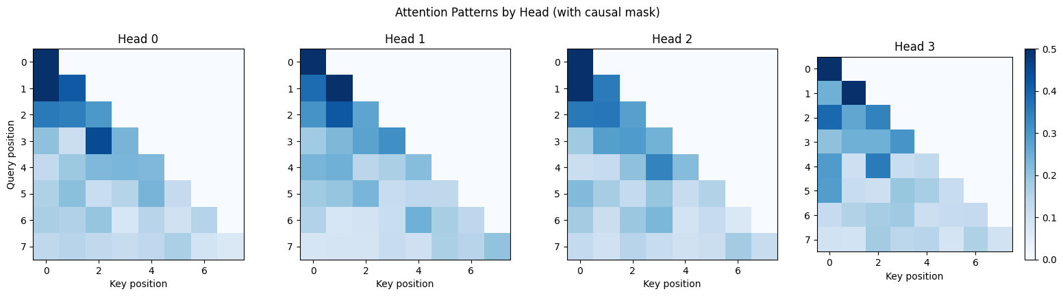

Note: These are random (untrained) weights.
In a trained model, each head would show distinct patterns.

What Trained Heads Learn¶

Research on trained transformers has identified several common head types:

Pattern	What It Does	Example
Previous token	Always attends to position $i-1$	Bigram-like patterns
Beginning of sequence	Attends to first token	Often a “null” or default attention
Positional	Attends to specific relative positions	Fixed offsets
Induction	Copies patterns: if “AB...A” seen, attend to B	In-context learning
Syntactic	Subject-verb, noun-adjective	Grammar structure

The model figures out which patterns are useful during training. We don’t program them in—they emerge from the data.

The Output Projection¶

After concatenating head outputs, we apply one more linear transformation $W_O$ :

\text{output} = \text{Concat}(\text{head}_1, ..., \text{head}_h) W_O

(4)

Why this final projection?

Mixing information across heads: The concatenated output has information from all heads, but in separate “slots”. $W_O$ lets the model combine insights from different heads.
Learned recombination: Maybe head 0’s “subject” information should be combined with head 2’s “semantic” information. $W_O$ learns these combinations.
Consistent interface: The output has the same dimension as the input ( $d_{model}$ ), which is needed for residual connections.

# Parameter count
total_params = sum(p.numel() for p in mha.parameters())

print("Multi-Head Attention Parameters:")
print(f"  W_q: ({d_model}, {d_model}) = {d_model * d_model:,}")
print(f"  W_k: ({d_model}, {d_model}) = {d_model * d_model:,}")
print(f"  W_v: ({d_model}, {d_model}) = {d_model * d_model:,}")
print(f"  W_o: ({d_model}, {d_model}) = {d_model * d_model:,}")
print(f"  " + "-" * 30)
print(f"  Total: {total_params:,} parameters")
print()
print(f"That's 4 × d_model² = 4 × {d_model}² = {4 * d_model * d_model:,}")

Multi-Head Attention Parameters:
  W_q: (256, 256) = 65,536
  W_k: (256, 256) = 65,536
  W_v: (256, 256) = 65,536
  W_o: (256, 256) = 65,536
  ------------------------------
  Total: 262,144 parameters

That's 4 × d_model² = 4 × 256² = 262,144

Computational Complexity¶

Multi-head attention has the same computational complexity as single-head attention with the full dimension:

Single-head attention on $d_{model}$ dimensions:

Score computation: $O(n^2 \cdot d_{model})$

Multi-head attention with $h$ heads, each on $d_k = d_{model}/h$ dimensions:

Score computation per head: $O(n^2 \cdot d_k)$
Total: $h \times O(n^2 \cdot d_k) = O(n^2 \cdot d_{model})$

Same total compute, but multiple specialized views instead of one generic one.

Efficient Implementation: Fused Projections¶

In our implementation, we have separate $W_Q$ , $W_K$ , $W_V$ matrices. A common optimization is to fuse them into one matrix and split the output:

class MultiHeadAttentionFused(nn.Module):
    """
    Multi-head attention with fused QKV projection.
    
    More efficient: one matmul instead of three.
    """
    
    def __init__(self, d_model: int, num_heads: int, dropout: float = 0.1):
        super().__init__()
        assert d_model % num_heads == 0
        
        self.d_model = d_model
        self.num_heads = num_heads
        self.d_k = d_model // num_heads
        
        # Fused projection: computes Q, K, V in one matmul
        self.W_qkv = nn.Linear(d_model, 3 * d_model, bias=False)
        self.W_o = nn.Linear(d_model, d_model, bias=False)
        
        self.dropout = nn.Dropout(dropout)
    
    def forward(self, x: torch.Tensor, mask: torch.Tensor = None):
        batch_size, seq_len, _ = x.shape
        
        # Single projection, then split
        qkv = self.W_qkv(x)  # (batch, seq_len, 3 * d_model)
        qkv = qkv.view(batch_size, seq_len, 3, self.num_heads, self.d_k)
        qkv = qkv.permute(2, 0, 3, 1, 4)  # (3, batch, heads, seq, d_k)
        Q, K, V = qkv[0], qkv[1], qkv[2]
        
        # Attention (same as before)
        scores = torch.matmul(Q, K.transpose(-2, -1)) / math.sqrt(self.d_k)
        if mask is not None:
            scores = scores.masked_fill(mask, float('-inf'))
        
        attn = F.softmax(scores, dim=-1)
        attn = self.dropout(attn)
        
        context = torch.matmul(attn, V)
        context = context.transpose(1, 2).contiguous().view(batch_size, seq_len, self.d_model)
        
        return self.W_o(context), attn

# Compare parameter counts
mha_separate = MultiHeadAttention(256, 4)
mha_fused = MultiHeadAttentionFused(256, 4)

print(f"Separate projections: {sum(p.numel() for p in mha_separate.parameters()):,} params")
print(f"Fused projection: {sum(p.numel() for p in mha_fused.parameters()):,} params")
print("\nSame parameters, but fused is faster (one large matmul vs three)")

Separate projections: 262,144 params
Fused projection: 262,144 params

Same parameters, but fused is faster (one large matmul vs three)

How Many Heads?¶

The number of heads is a hyperparameter. Common choices:

Model	$d_{model}$	Heads	$d_k$
GPT-2 Small	768	12	64
GPT-2 Medium	1024	16	64
GPT-3	12288	96	128
LLaMA 7B	4096	32	128

Notice that $d_k$ stays relatively constant (64-128) across models. As $d_{model}$ grows, we add more heads rather than making each head larger.

Trade-offs:

More heads = more diverse patterns, but each head has less capacity
Fewer heads = more capacity per head, but less diversity

Empirically, having multiple heads helps significantly. Going from 1 to 8 heads is a big improvement; going from 8 to 32 is smaller but still beneficial.

Data Flow Summary¶

Input x: (batch, seq_len, d_model)
    │
    ├─→ W_q → Q ─┐
    ├─→ W_k → K ─┼─→ Reshape to (batch, num_heads, seq_len, d_k)
    └─→ W_v → V ─┘
                  │
                  ├─→ Head 0: Attention(Q₀, K₀, V₀) → out₀
                  ├─→ Head 1: Attention(Q₁, K₁, V₁) → out₁
                  ├─→ ...                           → ...
                  └─→ Head h: Attention(Qₕ, Kₕ, Vₕ) → outₕ
                                                     │
                              Concat: (batch, seq_len, d_model)
                                                     │
                                                   W_o
                                                     │
                              Output: (batch, seq_len, d_model)

The output has the same shape as the input—this is essential for residual connections.

Key Takeaways¶

Multiple heads capture different relationships in parallel
Each head operates on a subspace: $d_k = d_{model} / h$
Same computational cost as single-head attention
Output projection $W_O$ mixes information across heads
Different heads specialize in different patterns (syntactic, semantic, positional, etc.)

Next: Feed-Forward Networks¶

Attention is the “communication” layer—tokens gather information from each other. But we also need a “computation” layer to process that gathered information.

In the next notebook, we’ll implement the feed-forward network: a simple two-layer MLP that operates on each position independently. Despite its simplicity, it accounts for about 2/3 of the parameters in a transformer block.