Training at Scale - An Introduction to Transformers

We’ve built a complete transformer. Now comes the hard part: training it well.

Two problems immediately arise when you try to train on hobby hardware:

Memory constraints force us to use small batches, which makes training noisy
Overfitting means the model memorizes training data instead of learning patterns

This notebook introduces two techniques that solve these problems: gradient accumulation (for stable training with limited memory) and validation splits (for detecting overfitting).

The Batch Size Problem¶

Let’s start with a fundamental question: why does batch size matter?

During training, we compute the loss over a “batch” of examples, then update weights based on that loss. The gradient we compute is an estimate of the true gradient over the entire dataset:

\nabla_{\text{batch}} \approx \nabla_{\text{dataset}}

(1)

The statistical insight: Larger batches give better estimates. With a batch of 8, each example contributes 12.5% of the signal. One weird example can throw off the whole gradient. With a batch of 128, each example is just 0.8%—outliers get averaged out.

Batch Size	Gradient Noise	Training Stability
8	High	Erratic
32	Medium	Acceptable
128	Low	Smooth
512+	Very Low	Very smooth

The Memory Wall¶

So why not just use big batches? Memory.

During the forward pass, PyTorch stores activations at every layer (needed for backpropagation). For a transformer with:

6 layers, d_model=256, seq_len=128
Each activation: (batch, seq_len, d_model) floats

Memory per example:

\text{Memory} \approx \text{layers} \times \text{seq\_len} \times d_{\text{model}} \times 4 \text{ bytes}

(2)

= 6 \times 128 \times 256 \times 4 = 786\text{KB per example}

(3)

With batch size 8: ~6 MB. With batch size 128: ~100 MB. Add attention scores, gradients, optimizer states... it adds up fast!

On a laptop with 8GB RAM, you might max out at batch size 8-16. This creates a dilemma: we want large batches for stability but can’t fit them in memory.

Gradient Accumulation: The Solution¶

Here’s the key insight that saves us: gradients are additive.

If we compute gradients on two separate batches and add them together, we get the same result as computing gradients on one combined batch:

\nabla(L_1 + L_2) = \nabla L_1 + \nabla L_2

(4)

This means we can:

Process batch 1 → compute gradients → don’t update yet, just store
Process batch 2 → compute gradients → add to stored gradients
Repeat N times
Finally update weights with accumulated gradients

The result: We simulate a batch of size $N \times \text{batch\_size}$ while only ever holding one small batch in memory.

import torch
import torch.nn as nn
import torch.nn.functional as F
import matplotlib.pyplot as plt
import numpy as np

# Simple model and data for demonstration
model = nn.Linear(64, 10)
optimizer = torch.optim.AdamW(model.parameters(), lr=1e-3)

def get_batch(batch_size=8):
    """Generate random classification data."""
    x = torch.randn(batch_size, 64)
    y = torch.randint(0, 10, (batch_size,))
    return x, y

Standard Training (No Accumulation)¶

First, let’s see standard training where we update after every batch:

print("Standard training (batch_size=8, updates every batch):")
print("="*55)

losses = []
for step in range(8):
    x, y = get_batch(batch_size=8)
    
    # Forward pass
    logits = model(x)
    loss = F.cross_entropy(logits, y)
    
    # Backward pass
    loss.backward()
    
    # Update weights immediately
    optimizer.step()
    optimizer.zero_grad()
    
    losses.append(loss.item())
    print(f"Step {step}: loss = {loss.item():.4f} → update weights")

print(f"\nLoss variance: {np.var(losses):.4f} (high = noisy training)")

Standard training (batch_size=8, updates every batch):
=======================================================
Step 0: loss = 2.8670 → update weights
Step 1: loss = 2.4275 → update weights
Step 2: loss = 2.1647 → update weights
Step 3: loss = 2.6930 → update weights
Step 4: loss = 2.5277 → update weights
Step 5: loss = 2.6354 → update weights
Step 6: loss = 2.1532 → update weights
Step 7: loss = 2.6031 → update weights

Loss variance: 0.0549 (high = noisy training)

Training with Gradient Accumulation¶

Now let’s accumulate gradients over 4 batches before updating. This simulates an effective batch size of 32 (4 × 8):

# Reset model
model = nn.Linear(64, 10)
optimizer = torch.optim.AdamW(model.parameters(), lr=1e-3)

accumulation_steps = 4  # Accumulate over 4 mini-batches
batch_size = 8
effective_batch_size = accumulation_steps * batch_size  # = 32

print(f"Gradient accumulation (batch_size={batch_size}, accumulation_steps={accumulation_steps}):")
print(f"Effective batch size: {effective_batch_size}")
print("="*55)

accumulated_losses = []
optimizer.zero_grad()  # Start with zero gradients

for step in range(8):
    x, y = get_batch(batch_size=8)
    
    # Forward pass
    logits = model(x)
    loss = F.cross_entropy(logits, y)
    
    # CRITICAL: Scale loss by accumulation steps!
    # This ensures the final gradient magnitude matches a true large batch
    scaled_loss = loss / accumulation_steps
    scaled_loss.backward()  # Gradients accumulate (add to existing)
    
    accumulated_losses.append(loss.item())
    
    # Only update every accumulation_steps batches
    if (step + 1) % accumulation_steps == 0:
        optimizer.step()
        optimizer.zero_grad()  # Reset gradients for next accumulation
        avg_loss = np.mean(accumulated_losses[-accumulation_steps:])
        print(f"Step {step}: avg_loss = {avg_loss:.4f} → update weights")
    else:
        print(f"Step {step}: loss = {loss.item():.4f} → accumulating...")

Gradient accumulation (batch_size=8, accumulation_steps=4):
Effective batch size: 32
=======================================================
Step 0: loss = 2.6713 → accumulating...
Step 1: loss = 2.2812 → accumulating...
Step 2: loss = 2.7019 → accumulating...
Step 3: avg_loss = 2.4725 → update weights
Step 4: loss = 2.6787 → accumulating...
Step 5: loss = 2.6121 → accumulating...
Step 6: loss = 2.5706 → accumulating...
Step 7: avg_loss = 2.5733 → update weights

Why Scale the Loss?¶

Notice we divided the loss by accumulation_steps. Here’s why:

With a single batch of size $B$ , the loss is typically averaged:

L = \frac{1}{B} \sum_{i=1}^{B} \ell_i

(5)

If we accumulate over $N$ batches without scaling:

L_{\text{accumulated}} = \sum_{j=1}^{N} \frac{1}{B} \sum_{i=1}^{B} \ell_{ij} = \frac{N}{B} \sum_{\text{all}} \ell

(6)

That’s $N$ times too large! The gradients would be $N$ times what they’d be with a true batch of size $N \times B$ .

By dividing each loss by $N$ , we get:

L_{\text{correct}} = \frac{1}{N \cdot B} \sum_{\text{all}} \ell

(7)

Which is exactly the average over all $N \cdot B$ examples.

Validation: Detecting Overfitting¶

Now for the second problem: how do we know if our model is actually learning vs. just memorizing?

The Memorization Problem¶

Imagine a student preparing for an exam:

Memorization: They memorize exact answers to practice problems. On the exam, they fail because the questions are slightly different.
Understanding: They learn the underlying concepts. On the exam, they can solve new variations.

Neural networks face the same challenge. A model might achieve 0% error on training data by “memorizing” each example, yet fail completely on new data. This is overfitting.

The Validation Split¶

The solution is simple: hold out some data the model never sees during training.

Split	Purpose	Model Sees It?
Training (90%)	Learning weights	Yes, repeatedly
Validation (10%)	Monitoring generalization	Never during training

After each epoch, we evaluate on the validation set. If the model is truly learning patterns (not memorizing), it should perform well on both sets.

Interpreting Training Curves¶

By plotting training loss and validation loss over time, we can diagnose what’s happening:

epochs = np.arange(1, 21)

# Scenario 1: Healthy training (both losses decrease together)
train_healthy = 5.0 * np.exp(-0.15 * epochs) + 1.5
val_healthy = 5.2 * np.exp(-0.14 * epochs) + 1.7

# Scenario 2: Underfitting (both losses stay high)
train_underfit = 5.0 * np.exp(-0.03 * epochs) + 3.5
val_underfit = 5.2 * np.exp(-0.025 * epochs) + 3.8

# Scenario 3: Overfitting (validation rises while training falls)
train_overfit = 5.0 * np.exp(-0.2 * epochs) + 0.3
val_overfit = np.concatenate([
    5.2 * np.exp(-0.15 * epochs[:7]) + 2.0,
    np.linspace(2.6, 4.5, 13)
])

fig, axes = plt.subplots(1, 3, figsize=(15, 4))

# Healthy
axes[0].plot(epochs, train_healthy, 'b-', label='Training', linewidth=2)
axes[0].plot(epochs, val_healthy, 'r--', label='Validation', linewidth=2)
axes[0].set_title('Healthy Training', fontsize=12, fontweight='bold')
axes[0].set_xlabel('Epoch')
axes[0].set_ylabel('Loss')
axes[0].legend()
axes[0].grid(True, alpha=0.3)
axes[0].set_ylim(0, 6)

# Underfitting
axes[1].plot(epochs, train_underfit, 'b-', label='Training', linewidth=2)
axes[1].plot(epochs, val_underfit, 'r--', label='Validation', linewidth=2)
axes[1].set_title('Underfitting', fontsize=12, fontweight='bold')
axes[1].set_xlabel('Epoch')
axes[1].legend()
axes[1].grid(True, alpha=0.3)
axes[1].set_ylim(0, 6)

# Overfitting
axes[2].plot(epochs, train_overfit, 'b-', label='Training', linewidth=2)
axes[2].plot(epochs, val_overfit, 'r--', label='Validation', linewidth=2)
axes[2].axvline(x=7, color='orange', linestyle=':', linewidth=2, label='Overfitting starts')
axes[2].set_title('Overfitting', fontsize=12, fontweight='bold')
axes[2].set_xlabel('Epoch')
axes[2].legend()
axes[2].grid(True, alpha=0.3)
axes[2].set_ylim(0, 6)

plt.tight_layout()
plt.show()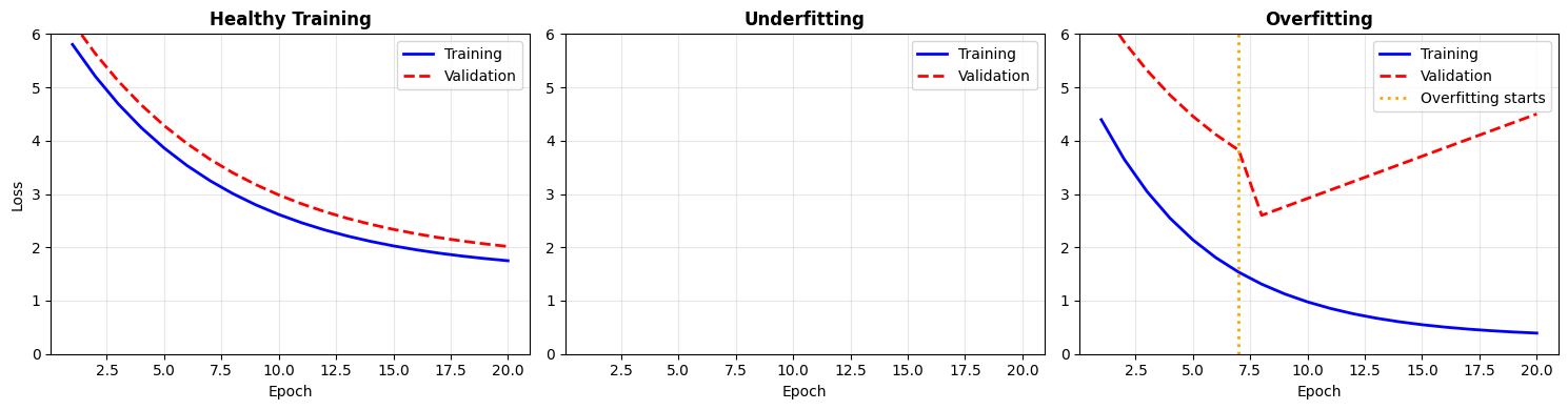

Diagnostic Guide¶

Pattern	Diagnosis	Solution
Both losses decrease together	Healthy	Keep training
Both losses stay high	Underfitting	Larger model, more training
Train ↓, Val ↑	Overfitting	More data, regularization, early stopping
Large gap (train << val)	Overfitting	Same as above
Training loss spikes	Unstable	Lower learning rate

Complete Training Loop¶

Let’s put it all together—a training loop with gradient accumulation and validation monitoring:

def train_with_validation(
    model,
    train_data,
    val_data,
    optimizer,
    epochs,
    accumulation_steps=1,
    device='cpu'
):
    """
    Training loop with gradient accumulation and validation.
    
    Args:
        model: The transformer model
        train_data: DataLoader for training set
        val_data: DataLoader for validation set
        optimizer: Optimizer (e.g., AdamW)
        epochs: Number of training epochs
        accumulation_steps: Number of batches to accumulate
        device: 'cpu' or 'cuda'
    
    Returns:
        Dictionary with training history
    """
    history = {'train_loss': [], 'val_loss': []}
    
    for epoch in range(epochs):
        # ===== Training Phase =====
        model.train()  # Enable dropout, batch norm training mode
        train_loss = 0
        num_batches = 0
        optimizer.zero_grad()
        
        for step, (x, y) in enumerate(train_data):
            x, y = x.to(device), y.to(device)
            
            # Forward pass
            logits = model(x)
            loss = F.cross_entropy(logits, y)
            
            # Scale and accumulate gradients
            scaled_loss = loss / accumulation_steps
            scaled_loss.backward()
            
            train_loss += loss.item()
            num_batches += 1
            
            # Update weights every accumulation_steps batches
            if (step + 1) % accumulation_steps == 0:
                optimizer.step()
                optimizer.zero_grad()
        
        # Handle remaining gradients if batches don't divide evenly
        if num_batches % accumulation_steps != 0:
            optimizer.step()
            optimizer.zero_grad()
        
        avg_train_loss = train_loss / num_batches
        history['train_loss'].append(avg_train_loss)
        
        # ===== Validation Phase =====
        model.eval()  # Disable dropout, use running stats for batch norm
        val_loss = 0
        num_val_batches = 0
        
        with torch.no_grad():  # No gradient computation (faster, saves memory)
            for x, y in val_data:
                x, y = x.to(device), y.to(device)
                logits = model(x)
                loss = F.cross_entropy(logits, y)
                val_loss += loss.item()
                num_val_batches += 1
        
        avg_val_loss = val_loss / num_val_batches
        history['val_loss'].append(avg_val_loss)
        
        # Report progress
        print(f"Epoch {epoch+1}/{epochs}: "
              f"train_loss={avg_train_loss:.4f}, "
              f"val_loss={avg_val_loss:.4f}")
        
        # Early warning for overfitting
        if len(history['val_loss']) > 1:
            if history['val_loss'][-1] > history['val_loss'][-2] * 1.05:
                print("  ⚠️  Warning: validation loss increased!")
    
    return history

# Demonstrate the training loop structure
print("Training Loop Structure:")
print("="*50)
print("""
for epoch in range(epochs):
    
    # 1. TRAINING PHASE
    model.train()              # Enable training mode
    optimizer.zero_grad()      # Clear old gradients
    
    for step, batch in enumerate(train_data):
        loss = compute_loss(model, batch)
        (loss / accum_steps).backward()  # Accumulate
        
        if (step + 1) % accum_steps == 0:
            optimizer.step()   # Update weights
            optimizer.zero_grad()
    
    # 2. VALIDATION PHASE
    model.eval()               # Disable training mode
    
    with torch.no_grad():      # No gradients needed
        for batch in val_data:
            loss = compute_loss(model, batch)
            # Just record loss, don't update anything
    
    # 3. MONITOR AND LOG
    print(f"Epoch {epoch}: train={train_loss}, val={val_loss}")
""")

Training Loop Structure:
==================================================

for epoch in range(epochs):

    # 1. TRAINING PHASE
    model.train()              # Enable training mode
    optimizer.zero_grad()      # Clear old gradients

    for step, batch in enumerate(train_data):
        loss = compute_loss(model, batch)
        (loss / accum_steps).backward()  # Accumulate

        if (step + 1) % accum_steps == 0:
            optimizer.step()   # Update weights
            optimizer.zero_grad()

    # 2. VALIDATION PHASE
    model.eval()               # Disable training mode

    with torch.no_grad():      # No gradients needed
        for batch in val_data:
            loss = compute_loss(model, batch)
            # Just record loss, don't update anything

    # 3. MONITOR AND LOG
    print(f"Epoch {epoch}: train={train_loss}, val={val_loss}")

Important Details¶

model.train() vs model.eval()¶

These mode switches matter for:

Dropout: Randomly zeros neurons during training (regularization), but we want deterministic predictions during validation
Batch Normalization: Uses batch statistics during training, running statistics during eval

Always use model.train() before training and model.eval() before validation!

torch.no_grad()¶

During validation, we don’t need gradients—we’re just measuring performance, not updating weights. torch.no_grad() tells PyTorch to skip gradient computation, which:

Runs faster (no backward graph construction)
Uses less memory (no activation storage)

Practical Recommendations¶

Based on typical hobby hardware (8-16GB RAM, consumer GPU or Apple Silicon):

Parameter	Recommended	Notes
Batch size	8-16	Whatever fits in memory
Accumulation steps	8-16	Effective batch 64-256
Validation split	10%	Or 5% for large datasets
Early stopping patience	3-5 epochs	Stop if val loss doesn’t improve

Memory-compute tradeoff: If you have more memory, use larger batches (faster). If memory is tight, use more accumulation steps (same quality, slower).

Effective improvements:

20-30% lower final loss from stable gradients
Smoother training curves, easier debugging
Confidence that your model generalizes
Works on commodity hardware!

Summary¶

Technique	Problem Solved	How It Works
Gradient Accumulation	Small batches → noisy training	Accumulate gradients over N batches, then update
Validation Split	Can’t detect overfitting	Hold out data to test generalization

Key formulas:

Gradient accumulation (scale loss):

L_{\text{scaled}} = \frac{L}{N} \quad \text{where } N = \text{accumulation steps}

(8)

Effective batch size:

B_{\text{effective}} = B_{\text{micro}} \times N

(9)

Next: KV-Cache¶

Training teaches the model what to predict. But how do we actually generate text efficiently? The naive approach recomputes everything for each token—wasteful! Next, we’ll see how KV-caching makes generation fast by reusing previous computations.