
You know what’s frustrating? Training a model for 12 hours, coming back with coffee in hand, and seeing “Loss: NaN” on your screen.
Hyperparameters matter. Like, really matter. The difference between a hyperparameter configuration that works and one that doesn’t isn’t subtle. it’s the difference between “my model is learning!” and “why is everything on fire?”
This notebook is your guide to tuning hyperparameters for SFT, DPO, and RLHF. We’ll explain what each knob does, why it matters, and how to avoid the common mistakes that make models sad.
The Stakes: Why Hyperparameters Matter
Let’s start with a reality check. Here’s what can happen with different hyperparameter choices:
Bad hyperparameters:
Step 100:  Loss = 2.5
Step 200:  Loss = 2.3  (okay, moving in the right direction...)
Step 300:  Loss = 2.4  (wait, it went up?)
Step 400:  Loss = 2.6  (this is bad)
Step 500:  Loss = NaN  (everything is on fire)
Good hyperparameters:
Step 100:  Loss = 2.5
Step 200:  Loss = 1.8  (nice!)
Step 300:  Loss = 1.4  (getting better)
Step 400:  Loss = 1.2  (smooth sailing)
Step 500:  Loss = 1.1  (we have a winner)
Same model. Same data. Different hyperparameters.
The good news? You don’t need to guess randomly. There are patterns, heuristics, and rules of thumb that work across different models and tasks. That’s what we’re here to learn.
Learning Rate: The King of Hyperparameters
If you only tune one hyperparameter, make it the learning rate.
What is it? The learning rate controls how big of a step your optimizer takes when updating model weights. Think of it like this: you’re hiking down a mountain in the fog (the fog is the loss landscape, stay with me). The learning rate is how big your steps are.
Too high: You take huge steps, overshoot the valley, and bounce around like a pinball. Eventually you might bounce right off the mountain (Loss = NaN).
Too low: You take tiny, shuffling steps. You’re technically making progress, but you’ll die of old age before reaching the bottom.
Just right: Nice, confident steps that make steady progress toward the minimum.
Here’s the tricky part: the “right” learning rate depends on what you’re doing.
Learning Rates for SFT (Supervised Fine-Tuning)
When you’re doing supervised fine-tuning, your model is already pre-trained. The weights are already pretty good! You just need to nudge them in the right direction. Small, gentle nudges.
| Setup | Learning Rate | Why? |
|---|---|---|
| Full fine-tuning | 2e-5 to 5e-5 | Model already knows language, small updates preserve that knowledge |
| LoRA (r=8-16) | 1e-4 to 5e-4 | LoRA parameters start random, need stronger updates to learn anything |
| LoRA (r=32-64) | 5e-5 to 2e-4 | Higher capacity = more parameters = more stable training |
Notice something? LoRA uses a higher learning rate than full fine-tuning. This trips people up constantly. “Wait, I thought lower learning rates were safer?” They are! But LoRA’s low-rank matrices start from random initialization. You need a bigger learning rate to get them moving.
Learning Rates for DPO (Direct Preference Optimization)
DPO is.. sensitive. Like, really sensitive. You’re not teaching the model new tasks, you’re adjusting its preferences between similar outputs. This requires a delicate touch.
| Setup | Learning Rate | Why? |
|---|---|---|
| Full fine-tuning | 5e-6 to 2e-5 | Tiny changes to preferences, don’t want to break the model |
| LoRA (r=8-16) | 5e-5 to 2e-4 | Random init again, need stronger signal |
Notice DPO’s learning rates are roughly 5-10x lower than SFT for the same setup. That’s because the preference signal is subtle. if you use a huge learning rate, you’ll overfit to your preference data and make the model weird.
Learning Rates for RLHF (Reinforcement Learning from Human Feedback)
RLHF with PPO is the most sensitive of all. You’re doing reinforcement learning now, which is inherently unstable (thanks, policy gradients). Lower learning rates = better sleep at night.
| Component | Learning Rate | Why? |
|---|---|---|
| Policy (full FT) | 1e-6 to 5e-6 | RL is unstable, tiny steps keep things smooth |
| Policy (LoRA) | 1e-5 to 5e-5 | LoRA more stable, can go a bit higher |
| Value network | 3e-5 to 1e-4 | Separate network, doesn’t affect generation, can train faster |
The value network gets a higher learning rate because it’s a separate network that just predicts values. it doesn’t directly affect what your model says, so you can be a bit more aggressive with training it.
Learning Rate Range Test
Here’s a handy tool when you’re not sure what learning rate to use. The idea: gradually increase the learning rate and watch what happens to the loss.
At first (low LR): loss decreases slowly
Sweet spot (optimal LR): loss decreases quickly (this is what we want!)
Too high: loss stops decreasing or starts increasing
We want to find the LR where the loss is decreasing the fastest. That’s usually a good starting point for training.
import torch
import numpy as np

def lr_range_test(model, dataloader, min_lr=1e-6, max_lr=1e-3, steps=100):
    """Run learning rate range test to find optimal LR."""
    lrs = []
    losses = []

    # Exponentially increase LR from min_lr to max_lr
    lr_mult = (max_lr / min_lr) ** (1 / steps)
    lr = min_lr

    optimizer = torch.optim.AdamW(model.parameters(), lr=lr)

    for i, batch in enumerate(dataloader):
        if i >= steps:
            break

        # Forward pass
        loss = model(**batch).loss

        # Record
        lrs.append(lr)
        losses.append(loss.item())

        # Backward
        optimizer.zero_grad()
        loss.backward()
        optimizer.step()

        # Increase learning rate for next iteration
        lr *= lr_mult
        for param_group in optimizer.param_groups:
            param_group['lr'] = lr

    # Find LR with steepest negative gradient (fastest loss decrease)
    gradients = np.gradient(losses)
    best_idx = np.argmin(gradients)
    optimal_lr = lrs[best_idx]

    print(f"Suggested learning rate: {optimal_lr:.2e}")
    print(f"  (This is where loss decreased fastest)")
    return optimal_lr, lrs, losses
Usage:
optimal_lr, lrs, losses = lr_range_test(model, dataloader)
plt.plot(lrs, losses)
plt.xscale('log')
plt.show()
Learning Rate Schedules: The Journey Matters
Okay, so you’ve picked a learning rate. Great! But you probably don’t want to use the same learning rate for the entire training run.
Think about it like driving. When you’re pulling out of your driveway, you start slow (warmup). Then you accelerate to highway speed (peak learning rate). As you approach your destination, you slow down (decay). You don’t just slam the gas pedal and hold it there the whole time.
(Well, you could, but that’s how you end up overshooting your exit.)
Learning Rate Schedules: Your Options
1. COSINE WITH WARMUP (Recommended)
This is the standard choice. Here’s what happens:
Steps 0-100: Linear warmup (0 → peak_lr)
Gently ease into training, stabilizes early steps
Steps 100-1000: Cosine decay (peak_lr → ~0.1 × peak_lr)
Smooth slowdown as we approach the end
Why cosine? It’s smooth (no sudden changes) and it naturally slows down as you get closer to convergence.
2. LINEAR DECAY
Steps 0-100: Linear warmup
Steps 100-1000: Linear decay to 0
This works, but the constant decay rate can be too aggressive early on and too gentle later.
3. CONSTANT WITH WARMUP
Steps 0-100: Linear warmup
Steps 100+: Constant at peak_lr
Use this for short training runs where you don’t want the LR to decay. Less common these days.
Warmup: How Many Steps?
Rule of thumb: 5-10% of total training steps
Examples:
Short training (1,000 steps): warmup = 50-100
Medium training (10,000 steps): warmup = 500-1,000
Long training (100,000 steps): warmup = 2,000-5,000
Why warmup? At the start of training, gradients can be unstable. Starting with a low LR and ramping up gives the model a chance to stabilize before taking big steps.
Code example:
from transformers import get_cosine_schedule_with_warmup

scheduler = get_cosine_schedule_with_warmup(
    optimizer,
    num_warmup_steps=100,
    num_training_steps=1000,
)
Batch Size: More Than Just a Memory Constraint
People think of batch size as “how much fits in my GPU.” And sure, that’s part of it. But batch size actually affects how your model learns.
What is batch size? It’s how many examples you process before updating the model’s weights. A batch size of 8 means: look at 8 examples, compute gradients for all of them, average those gradients together, then take one optimization step.
The Effective Batch Size
The effective batch size is what actually matters:
effective_batch_size = batch_size × gradient_accumulation_steps × num_gpusGradient accumulation is a clever trick. If you can only fit 4 examples in memory, but you want an effective batch of 32, you can:
Process 4 examples, compute gradients (but don’t update weights yet)
Process 4 more examples, add their gradients to the first batch
Repeat 8 times total (4 × 8 = 32)
Now update the weights
Same effective batch size, fits in less memory. Neat!
Recommended Batch Sizes
| Method | Effective Batch | Typical Physical Batch | Why? |
|---|---|---|---|
| SFT | 32-128 | 8-16 per GPU | Stable gradients, good throughput |
| DPO | 16-64 | 4-8 per GPU | Each example is chosen+rejected pair (2x memory!) |
| RLHF | 16-64 | 4-8 per GPU | RL is unstable, smaller batches help |
| Reward Model | 32-64 | 8-16 per GPU | Comparison task, benefits from variety |
Notice DPO uses smaller batches. That’s because each training example is actually two completions (the chosen one and the rejected one), so it takes twice the memory.
Batch Size → Learning Rate Scaling
If you change your batch size, you should probably change your learning rate too.
Why? Larger batches give smoother (less noisy) gradients. Smoother gradients mean you can take bigger steps without things going haywire.
Two schools of thought:
LINEAR SCALING: If you double the batch size, double the LR
Theory: You’re doing the same amount of work, just in bigger chunks
Practice: Can be aggressive, sometimes causes instability
SQRT SCALING: If you double the batch size, multiply LR by √2 ≈ 1.4
Theory: Accounts for noise reduction without being too aggressive
Practice: More conservative, usually safer
When in doubt, use sqrt scaling. It’s the safer bet.
import numpy as np

def scale_learning_rate(base_lr, base_batch, new_batch, method='sqrt'):
    """Scale learning rate when changing batch size."""
    if method == 'linear':
        scaled_lr = base_lr * (new_batch / base_batch)
        print(f"  Using linear scaling: LR × {new_batch / base_batch:.2f}")
    elif method == 'sqrt':
        scaling_factor = np.sqrt(new_batch / base_batch)
        scaled_lr = base_lr * scaling_factor
        print(f"  Using sqrt scaling: LR × {scaling_factor:.2f}")
    else:
        raise ValueError(f"Unknown method: {method}")

    return scaled_lr
Example: You found a good LR for batch size 32, but now you want to use batch size 64
Starting point: batch_size=32, lr=3e-4
Scaling to batch_size=64:
Sqrt scaling:
lr=4.24e-4(multiply by √2 ≈ 1.41)Linear scaling:
lr=6e-4(multiply by 2)
Scaling to batch_size=128:
Sqrt scaling:
lr=6e-4(multiply by √4 = 2)Linear scaling:
lr=1.2e-3(multiply by 4)
Recommendation: Start with sqrt scaling. If training is too slow, try linear scaling (but watch for instability).
DPO Beta: The Preference Strength Knob
Alright, time for the DPO-specific hyperparameter that causes the most confusion: beta.
Remember the DPO loss function? Here it is:
That controls how strongly you push the model to prefer the chosen response over the rejected one.
What does beta do?
Low beta (0.01-0.05): Gentle nudges. “Hey model, maybe prefer this response a little bit more?”
Medium beta (0.1-0.3): Standard. “I’d like you to clearly prefer the chosen response.”
High beta (0.5-1.0): Aggressive. “YOU WILL PREFER THIS RESPONSE OR ELSE.”
Higher beta = stronger preference signal = more risk of overfitting to your preference data.
How to Choose Beta
The key question: How much do you trust your preference data?
| Data Quality | Beta Range | Reasoning |
|---|---|---|
| High (human annotations, clear preferences) | 0.1-0.3 | Trust your data, use it! |
| Medium (AI-labeled, decent quality) | 0.05-0.1 | Some noise, be gentle |
| Low (heuristics, noisy labels) | 0.01-0.05 | Don’t overfit to noise |
If your preference data is “Response A uses proper grammar and Response B is gibberish,” you can use a higher beta. If your preference data is “Response A is slightly better according to this AI judge that might be hallucinating,” maybe go lower.
import matplotlib.pyplot as plt
import numpy as np

# Visualize the effect of beta on the loss function
margin_range = np.linspace(-5, 5, 100)

plt.figure(figsize=(12, 6))

# Plot DPO loss for different beta values
for beta in [0.01, 0.1, 0.3, 1.0]:
    # The margin is: log(π/π_ref) for chosen - log(π/π_ref) for rejected
    # Positive margin = model prefers chosen (good!)
    # Negative margin = model prefers rejected (bad!)

    logits = beta * margin_range
    loss = -np.log(1 / (1 + np.exp(-logits)))  # This is -log(sigmoid(logits))
    plt.plot(margin_range, loss, label=f'beta={beta}', linewidth=2)

plt.xlabel('Log Ratio Margin (chosen - rejected)', fontsize=12)
plt.ylabel('DPO Loss', fontsize=12)
plt.title('How Beta Affects DPO Loss', fontsize=14, fontweight='bold')
plt.axvline(x=0, color='black', linestyle='--', alpha=0.3, label='No preference')
plt.legend(fontsize=10)
plt.grid(True, alpha=0.3)
plt.tight_layout()
plt.show()

print("What this plot tells us:")
print("=" * 60)
print()
print("X-axis (margin): How much the model prefers chosen over rejected")
print("  Positive = model prefers chosen (good!)")
print("  Negative = model prefers rejected (bad!)")
print()
print("Y-axis (loss): How much we penalize the model")
print()
print("Notice:")
print("  • Higher beta = steeper curve = stronger penalty for mistakes")
print("  • beta=0.01 is almost flat (gentle corrections)")
print("  • beta=1.0 is very steep (harsh penalties)")
print()
print("Rule of thumb:")
print("  Start with beta=0.1")
print("  If model isn't learning preferences → increase beta")
print("  If model is overfitting to preferences → decrease beta")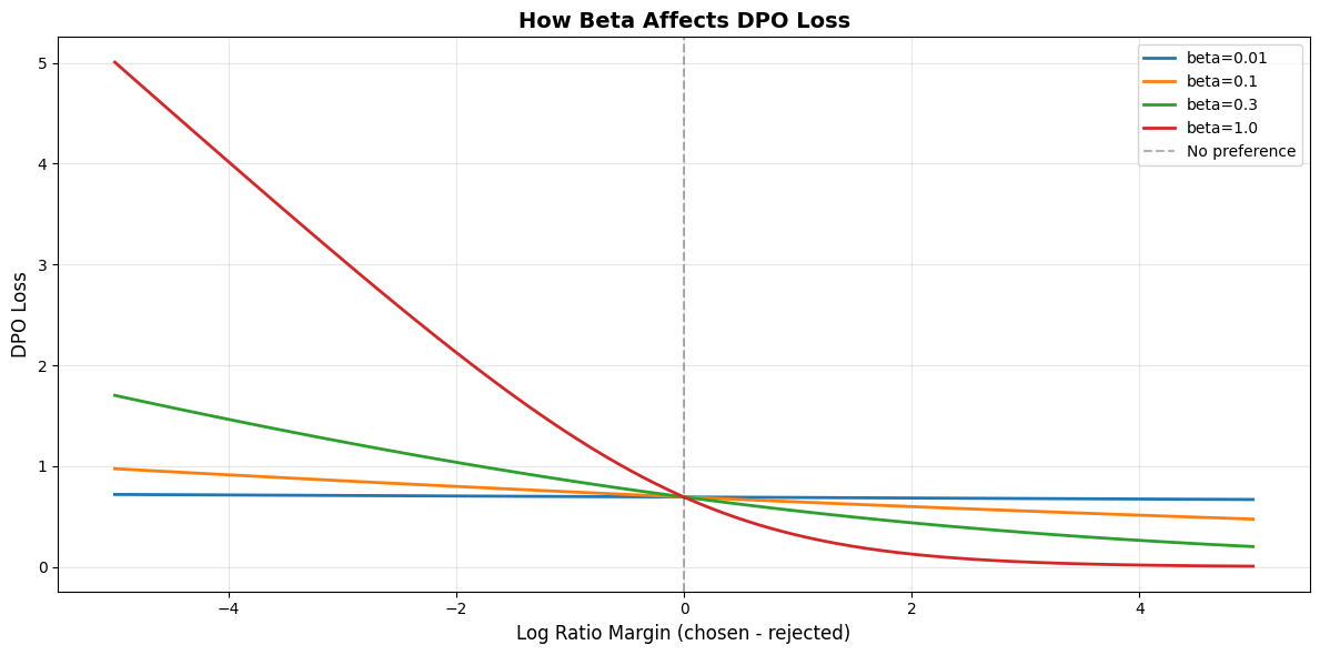
What this plot tells us:
============================================================

X-axis (margin): How much the model prefers chosen over rejected
  Positive = model prefers chosen (good!)
  Negative = model prefers rejected (bad!)

Y-axis (loss): How much we penalize the model

Notice:
  • Higher beta = steeper curve = stronger penalty for mistakes
  • beta=0.01 is almost flat (gentle corrections)
  • beta=1.0 is very steep (harsh penalties)

Rule of thumb:
  Start with beta=0.1
  If model isn't learning preferences → increase beta
  If model is overfitting to preferences → decrease beta
RLHF: The KL Divergence Leash
If you’re doing RLHF (reinforcement learning from human feedback) with PPO, you have a different problem: your policy model might go completely off the rails chasing reward.
Imagine you have a reward model that gives high scores for helpful responses. Without any constraints, your policy might discover that repeating “This is helpful! This is helpful! This is helpful!” 500 times gets a high reward score. Technically the reward model likes it.. but it’s not actually useful.
(This happens. Like, a lot.)
The KL divergence constraint is your safety leash. It penalizes the policy for deviating too far from the reference model (usually the SFT model):
That (often called kl_coef) controls how tight the leash is.
Low KL coef (0.01): Long leash. Policy can wander far from reference. Risky!
Medium KL coef (0.1): Standard leash. Balanced exploration and safety.
High KL coef (0.5-2.0): Short leash. Policy stays close to reference. Safe but limiting.
The goal is to improve on the reference model without going weird. Too loose and you get gibberish. Too tight and you don’t improve at all.
Adaptive KL Controller
Instead of picking a fixed KL coefficient and hoping it’s right, we can adapt it during training based on what’s happening.
The idea:
Set a target KL divergence (how much deviation you’re comfortable with)
If actual KL is too high → increase the coefficient (tighten the leash)
If actual KL is too low → decrease the coefficient (loosen the leash)
This way, the KL coefficient automatically adjusts to keep you in the sweet spot between “too conservative” and “completely unhinged.”
class AdaptiveKLController:
    """Adaptive KL coefficient for RLHF."""

    def __init__(self, init_kl_coef=0.1, target_kl=0.01):
        self.kl_coef = init_kl_coef      # Starting coefficient
        self.target_kl = target_kl        # Target KL divergence

    def update(self, current_kl):
        """Adjust KL coefficient based on current KL divergence."""
        if current_kl > 2 * self.target_kl:
            # Model is diverging too much from reference
            self.kl_coef *= 1.5
        elif current_kl < 0.5 * self.target_kl:
            # Model is too conservative
            self.kl_coef *= 0.8

        return self.kl_coef
Example training run:
Step 1: KL = 0.025 (too high) → Increase coef to 0.150
Step 2: KL = 0.030 (too high) → Increase coef to 0.225
Step 3: KL = 0.012 (just right) → Keep coef at 0.225
Step 4: KL = 0.003 (too low) → Decrease coef to 0.180
Other important RLHF hyperparameters:
clip_epsilon (usually 0.2): PPO clips policy updates to prevent huge changes. Standard value is 0.2, don’t mess with it unless you know what you’re doing.
ppo_epochs (usually 4): How many optimization passes over each batch. More epochs = more sample efficient, but risk overfitting. 4 is a good balance.
LoRA: Rank and Alpha
When you’re using LoRA (Low-Rank Adaptation), you have two key hyperparameters to tune: rank (r) and alpha.
Quick refresher: LoRA doesn’t update the original model weights. Instead, it learns low-rank matrices that get added to the original weights. The rank determines how “expressive” these low-rank matrices can be.
Rank (r): The dimensionality of the low-rank decomposition
Higher rank = more parameters = more capacity = can learn more complex adaptations
Lower rank = fewer parameters = less capacity = faster and more memory-efficient
Alpha: A scaling factor applied to the LoRA updates
Think of it as the “learning strength” of the LoRA layers
Standard relationship:
alpha = 2 × rank
Here’s the thing: picking the right rank is a balancing act. Too low and your model can’t learn the task (underfitting). Too high and you’re wasting memory and computation without much benefit.
The sweet spot depends on your model size and task complexity.
LoRA Rank Selection Guide
| Model Size | Task Complexity | Rank | Alpha | % Trainable Params |
|---|---|---|---|---|
| <1B | Simple | 4-8 | 8-16 | ~0.1-0.2% |
| <1B | Complex | 8-16 | 16-32 | ~0.2-0.4% |
| 1B-7B | Simple | 8-16 | 16-32 | ~0.2-0.4% |
| 1B-7B | Complex | 16-32 | 32-64 | ~0.4-0.8% |
| 7B+ | Complex | 32-64 | 64-128 | ~0.8-1.6% |
Standard relationship: alpha = 2 × rank
What do these ranks actually mean?
r=4: MINIMAL capacity
Good for: Very simple tasks (format changes, style tweaks)
~0.1% of full model parameters
Example: Teaching the model to use a specific format
r=8: LOW capacity
Good for: Simple domain adaptation, basic instructions
~0.2% of full model parameters
Example: Fine-tuning for customer service responses
r=16: STANDARD capacity
Good for: Most tasks, general-purpose fine-tuning
~0.4% of full model parameters
Example: Domain-specific QA, instruction following
→ This is the default you should probably start with
r=32: HIGH capacity
Good for: Complex reasoning, specialized domains
~0.8% of full model parameters
Example: Medical/legal QA, complex code generation
r=64: VERY HIGH capacity
Good for: When r=32 isn’t enough (rare)
~1.6% of full model parameters
Example: Highly specialized scientific tasks
Start with r=16, alpha=32
Too easy → model converges too fast → try lower rank
Too hard → model struggles to learn → try higher rank
Most of the time, r=16 is perfectly fine. Don’t overthink it!
Hyperparameter Cheat Sheet: Your Quick Reference
Alright, we’ve covered a lot. Let’s consolidate this into some practical, copy-pasteable configurations that actually work.
These are battle-tested starting points. Will they be perfect for your exact use case? Probably not. But they’ll get you 90% of the way there, and you can tune from there.
Configuration Cheat Sheet
Quick reference configurations that actually work. These are battle-tested starting points that’ll get you 90% of the way there.
SFT (Supervised Fine-Tuning) with LoRA
SFTConfig(
    learning_rate=3e-4,              # Higher for LoRA (random init)
    batch_size=8,                    # Fits most GPUs
    gradient_accumulation_steps=4,   # → effective batch = 32
    num_epochs=3,                    # 3-5 for most datasets
    warmup_steps=100,                # ~10% of training steps
    lr_scheduler_type="cosine",      # Smooth decay
    max_grad_norm=1.0,               # Gradient clipping
    weight_decay=0.01,               # Standard regularization
)

# LoRA config:
# - rank=16, alpha=32 for most tasks
# - rank=32, alpha=64 for complex tasks
# - rank=8, alpha=16 if memory-constrained
DPO (Direct Preference Optimization) with LoRA
DPOConfig(
    learning_rate=5e-5,              # MUCH lower than SFT!
    beta=0.1,                        # Standard preference strength
    batch_size=4,                    # Each example = chosen + rejected
    gradient_accumulation_steps=8,   # → effective batch = 32
    num_epochs=1,                    # Usually sufficient for DPO
    warmup_steps=50,                 # Shorter warmup
    lr_scheduler_type="cosine",
    max_grad_norm=1.0,
)

# Beta tuning:
# - Start with 0.1
# - Increase if model isn't learning preferences
# - Decrease if model is overfitting to preferences
RLHF (PPO) with LoRA
RLHFConfig(
    # Policy network (the language model)
    policy_lr=1e-5,                  # Very low for stability

    # Value network (predicts rewards)
    value_lr=5e-5,                   # Can be higher

    # KL divergence penalty
    kl_coef=0.1,                     # Keeps policy near reference
    target_kl=0.01,                  # Target KL divergence

    # PPO-specific
    clip_epsilon=0.2,                # Standard PPO clipping
    ppo_epochs=4,                    # Optimization passes per batch

    # Training
    batch_size=4,                    # Small for RL stability
    gradient_accumulation_steps=8,
    max_grad_norm=0.5,               # Stricter clipping for RL
)

# Use adaptive KL coefficient (see AdaptiveKLController above)
# to automatically adjust kl_coef during training
Quick Decision Guide
Pick your method (SFT, DPO, or RLHF)
Start with the config above
Adjust batch size to fit your GPU
If you change batch size, scale learning rate (see earlier)
Run a few hundred steps and watch the loss
Loss going down smoothly? Great, keep going!
Loss exploding (NaN)? Lower learning rate
Loss barely moving? Increase learning rate
Tune method-specific params (beta for DPO, kl_coef for RLHF)
That’s it. Don’t overthink it. These configs work.
Common Mistakes (And How to Avoid Them)
Let’s talk about the mistakes I see people make over and over again. Learn from our collective pain.
Mistake #1: Using the Same Learning Rate Everywhere
This is the big one. People find a learning rate that works for SFT and then use it for everything.
Bad:
# Nooooo!
sft_config = SFTConfig(learning_rate=3e-4)      # ✓ Good for SFT
dpo_config = DPOConfig(learning_rate=3e-4)      # ✗ Way too high!
rlhf_config = RLHFConfig(policy_lr=3e-4)        # ✗ Model will explode!
Good:
# Yes! Method-specific learning rates
sft_config = SFTConfig(learning_rate=3e-4)      # ✓ Standard for SFT
dpo_config = DPOConfig(learning_rate=5e-5)      # ✓ 5-10x lower
rlhf_config = RLHFConfig(policy_lr=1e-5)        # ✓ Even lower for RL
Why this matters: DPO and RLHF are much more sensitive than SFT. A learning rate that works fine for supervised learning will send your preference model into the stratosphere.
Mistake #2: Not Scaling Learning Rate for LoRA
LoRA uses randomly initialized matrices. They need a higher learning rate than pre-trained weights.
Bad:
# Using full fine-tuning LR with LoRA
config = SFTConfig(learning_rate=3e-5)  # ✗ Too low! LoRA will barely learn
Good:
# Higher LR for LoRA's random initialization
config = SFTConfig(learning_rate=3e-4)  # ✓ About 10x higher than full FT
Why this matters: With a too-low learning rate, LoRA will technically train, but it’ll take forever and might not reach good performance. You’ll waste hours wondering why your model isn’t learning.
Mistake #3: Skipping Warmup
Starting training with a high learning rate is like flooring the accelerator when your car is still in the driveway. Recipe for chaos.
Bad:
config = SFTConfig(
    learning_rate=3e-4,
    warmup_steps=0,  # ✗ No warmup = unstable start
)
Good:
config = SFTConfig(
    learning_rate=3e-4,
    warmup_steps=100,  # ✓ 5-10% of training steps
)
Why this matters: At the start of training, gradients can be large and unpredictable. Warmup gives the model a chance to stabilize before taking big steps. It’s especially important for LoRA, where those random matrices start with crazy gradients.
Mistake #4: Ignoring Effective Batch Size
“My batch size is 4” isn’t complete information. The effective batch size is what matters.
Misleading:
# These look the same, but they're not!
config_a = SFTConfig(batch_size=32, gradient_accumulation_steps=1)
config_b = SFTConfig(batch_size=4, gradient_accumulation_steps=8)
Both have effective batch size = 32, but:
Config A: Process 32 examples at once (high memory, one update)
Config B: Process 4 examples at a time, 8 accumulation steps (low memory, one update)
Why this matters: If you report “I used batch size 4” without mentioning gradient accumulation, others can’t reproduce your results. Always think in terms of effective batch size.
Mistake #5: Cranking Up Beta Without Good Data
High beta with noisy preference data is a disaster waiting to happen.
Bad:
# AI-generated preference labels (might be noisy)
dpo_config = DPOConfig(
    beta=1.0,  # ✗ Too aggressive for noisy data
)
Good:
# AI-generated preference labels (might be noisy)
dpo_config = DPOConfig(
    beta=0.05,  # ✓ Gentle, won't overfit to noise
)
Why this matters: Beta amplifies your preference signal. If that signal is noisy, high beta means “strongly overfit to garbage.” Start low, increase if needed.
The pattern here? Most mistakes come from copy-pasting configs without understanding what the hyperparameters actually do. Now you know better.
Summary: Your Hyperparameter Tuning Workflow
Let’s bring this all together into a practical workflow.
Step 1: Pick Your Starting Point
| Method | Learning Rate | Batch Size (effective) | Key Parameter |
|---|---|---|---|
| SFT (LoRA) | 3e-4 | 32-128 | rank=16 |
| DPO (LoRA) | 5e-5 | 16-64 | beta=0.1 |
| RLHF (LoRA) | 1e-5 | 16-64 | kl_coef=0.1 |
Step 2: Adjust for Your Hardware
Fit batch size to your GPU memory
Use gradient accumulation to reach target effective batch
Scale learning rate if you significantly change batch size (use sqrt scaling)
Step 3: Set Warmup and Schedule
Warmup steps = 5-10% of total training steps
Use cosine decay (it just works)
For short runs (<1000 steps), constant LR is fine
Step 4: Start Training and Watch Closely
Check loss after 50-100 steps
Loss smoothly decreasing? You’re good!
Loss stuck? Increase learning rate
Loss exploding? Decrease learning rate
Weird oscillations? Reduce batch size or increase warmup
Step 5: Tune Method-Specific Parameters
DPO: Adjust beta based on model behavior and data quality
RLHF: Use adaptive KL controller, watch for model collapse
LoRA: If model struggles, try higher rank
Tuning Priority:
Learning rate ← Start here! Biggest impact
Batch size ← For stability and speed
Method-specific ← Beta for DPO, KL for RLHF
Secondary ← Warmup, weight decay, clipping
Remember: these hyperparameters aren’t mysterious formulas. They’re knobs that control how your model learns. Understanding what each knob does means you can tune intelligently instead of randomly.
What’s Next?
Now you know how to tune hyperparameters without setting everything on fire. Nice!
But hyperparameters only matter if you can measure whether they’re working. And “loss going down” is just the start. there are much better ways to evaluate whether your model is actually getting better at the thing you care about.
That’s what we’ll cover next: comprehensive evaluation metrics that go beyond loss.