The Diffusion Transformer (DiT)

In the previous notebook, we built a working generative model using a CNN (U-Net). It successfully learned to transform noise into digits. But that architecture has fundamental limitations that become apparent at scale.

In this notebook, we replace the CNN with a Diffusion Transformer (DiT) - the same architecture that powers Stable Diffusion 3, Sora, and other state-of-the-art image and video generators.

Why Move Beyond CNNs?¶

CNNs process images through local convolution kernels:

Layer 1: Each pixel sees 3×3 = 9 neighbors
Layer 2: Each pixel sees 5×5 = 25 pixels  
Layer 3: Each pixel sees 7×7 = 49 pixels
  ...
Layer N: Receptive field grows linearly

To “see” the entire 28×28 image, you need many layers. Information must propagate step-by-step through the network, like a game of telephone.

Transformers take a different approach: every position can attend to every other position in a single layer.

Aspect	CNN (U-Net)	Transformer (DiT)
Receptive field	Local, grows with depth	Global from layer 1
Long-range dependencies	Requires many layers	Direct attention
Scaling behavior	Diminishing returns	Predictable improvement
Conditioning	Add/concatenate features	Modulate every operation

The key finding from the DiT paper: transformers follow scaling laws. Double the compute, get predictably better results. This is why modern image generators have switched to transformers.

What We’ll Build¶

By the end of this notebook, you’ll understand:

Patchification - Converting images to token sequences
Positional embeddings - Encoding 2D spatial structure
Self-attention - The mathematical heart of transformers
Adaptive Layer Norm (adaLN) - Superior timestep conditioning

import torch
import torch.nn as nn
import torchvision
import torchvision.transforms as transforms
from torch.utils.data import DataLoader
import matplotlib.pyplot as plt
import numpy as np

%load_ext autoreload
%autoreload 2

# Set up device
from from_noise_to_images import get_device
device = get_device()
print(f"Using device: {device}")

Using device: cuda

Step 1: Patchification - Images as Token Sequences¶

Transformers were designed for sequences - words in a sentence, tokens in code. To apply them to images, we need to convert the 2D pixel grid into a 1D sequence.

The Patchification Process¶

For an image $x \in \mathbb{R}^{H \times W \times C}$ with patch size $P$ :

Divide into patches: Split into $N = \frac{H}{P} \times \frac{W}{P}$ non-overlapping patches
Flatten each patch: Each patch becomes a vector of dimension $P^2 \cdot C$
Project to embedding space: Linear projection $E \in \mathbb{R}^{(P^2 C) \times D}$

\text{patches} = \text{Reshape}(x) \cdot E \in \mathbb{R}^{N \times D}

(1)

Concrete Example: Our MNIST Setup¶

For MNIST (28×28×1) with patch size 4:

Step	Calculation	Result
Number of patches	$\frac{28}{4} \times \frac{28}{4}$	$7 \times 7 = 49$ patches
Pixels per patch	$4 \times 4 \times 1$	16 values
Embedding dimension	(hyperparameter)	$D = 256$
Projection matrix	$E \in \mathbb{R}^{16 \times 256}$	4,096 parameters

The Computational Win¶

Self-attention has $O(N^2)$ complexity where $N$ is sequence length. Patches dramatically reduce this:

Approach	Sequence Length	Attention Cost
Pixel-level	$28 \times 28 = 784$	$784^2 = 614,656$
Patch-level (P=4)	$7 \times 7 = 49$	$49^2 = 2,401$
Speedup		256×

The tradeoff: larger patches = fewer tokens = faster, but lose fine detail within each patch. For small images like MNIST, $P=4$ strikes a good balance.

# Load MNIST
transform = transforms.Compose([
    transforms.ToTensor(),
    transforms.Normalize((0.5,), (0.5,))
])

train_dataset = torchvision.datasets.MNIST(
    root="./data",
    train=True,
    download=True,
    transform=transform
)

sample_img, label = train_dataset[0]
print(f"Image shape: {sample_img.shape}")
print(f"Label: {label}")

Image shape: torch.Size([1, 28, 28])
Label: 5

def visualize_patchification(img, patch_size=4):
    """
    Visualize the patchification process step by step.
    """
    img_display = (img[0] + 1) / 2  # Denormalize
    H, W = img_display.shape
    num_patches_h = H // patch_size
    num_patches_w = W // patch_size
    N = num_patches_h * num_patches_w
    
    fig, axes = plt.subplots(1, 4, figsize=(16, 4))
    
    # Original image
    axes[0].imshow(img_display.numpy(), cmap='gray')
    axes[0].set_title(f'Original: $x \\in \\mathbb{{R}}^{{{H}\\times{W}\\times1}}$', fontsize=11)
    axes[0].axis('off')
    
    # Image with patch grid
    axes[1].imshow(img_display.numpy(), cmap='gray')
    for i in range(1, num_patches_h):
        axes[1].axhline(y=i * patch_size - 0.5, color='red', linewidth=1)
    for j in range(1, num_patches_w):
        axes[1].axvline(x=j * patch_size - 0.5, color='red', linewidth=1)
    axes[1].set_title(f'Divide: $N = {num_patches_h}\\times{num_patches_w} = {N}$ patches', fontsize=11)
    axes[1].axis('off')
    
    # Extract and show patches as sequence
    patches = img_display.unfold(0, patch_size, patch_size).unfold(1, patch_size, patch_size)
    patches = patches.reshape(-1, patch_size, patch_size)
    
    patch_grid = torchvision.utils.make_grid(
        patches[:14].unsqueeze(1), nrow=7, padding=1, pad_value=0.5
    )
    axes[2].imshow(patch_grid[0].numpy(), cmap='gray')
    axes[2].set_title(f'Flatten: each patch $\\in \\mathbb{{R}}^{{{patch_size**2}}}$', fontsize=11)
    axes[2].axis('off')
    
    # Show embedding projection conceptually
    embed_dim = 256
    projection = np.random.randn(patch_size**2, embed_dim) * 0.1
    axes[3].imshow(projection, aspect='auto', cmap='RdBu', vmin=-0.3, vmax=0.3)
    axes[3].set_xlabel(f'Embedding dim ({embed_dim})')
    axes[3].set_ylabel(f'Patch pixels ({patch_size**2})')
    axes[3].set_title(f'Project: $E \\in \\mathbb{{R}}^{{{patch_size**2}\\times{embed_dim}}}$', fontsize=11)
    
    plt.suptitle('Patchification: Image to Sequence of Embeddings', fontsize=14)
    plt.tight_layout()
    plt.show()
    
    print(f"\nPatchification Summary:")
    print(f"  Input:  {H}×{W}×1 = {H*W} pixel values")
    print(f"  Patches: {N} patches, each {patch_size}×{patch_size} = {patch_size**2} pixels")
    print(f"  Output: {N} tokens, each {embed_dim}-dimensional")
    print(f"  Attention cost: {H*W}² = {(H*W)**2:,} → {N}² = {N**2:,} ({(H*W)**2 // N**2}× reduction)")

visualize_patchification(sample_img, patch_size=4)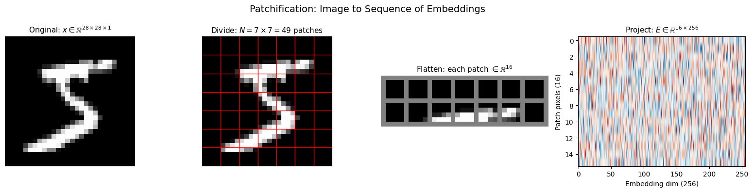


Patchification Summary:
  Input:  28×28×1 = 784 pixel values
  Patches: 49 patches, each 4×4 = 16 pixels
  Output: 49 tokens, each 256-dimensional
  Attention cost: 784² = 614,656 → 49² = 2,401 (256× reduction)

Step 2: Positional Embeddings - Encoding Spatial Structure¶

When we flatten patches into a sequence, we lose spatial information. The transformer sees:

[p_1, p_2, p_3, \ldots, p_{49}]

(2)

But it doesn’t know that $p_1$ is in the top-left corner and $p_{49}$ is in the bottom-right!

The Solution: Add Position Information¶

We add a positional embedding to each patch embedding:

z_i = p_i + \text{PE}(\text{row}_i, \text{col}_i)

(3)

Sinusoidal Positional Encoding¶

We use the sinusoidal encoding from “Attention Is All You Need”:

\text{PE}(\text{pos}, 2i) = \sin\left(\frac{\text{pos}}{10000^{2i/d}}\right)

(4)

\text{PE}(\text{pos}, 2i+1) = \cos\left(\frac{\text{pos}}{10000^{2i/d}}\right)

(5)

where $i$ is the dimension index and $d$ is the total embedding dimension.

Why Sinusoids Work¶

Property	Explanation
Unique encoding	Each position gets a distinct pattern
Relative positions	$\text{PE}(\text{pos}+k)$ is a linear function of $\text{PE}(\text{pos})$
Bounded values	All outputs in $[-1, 1]$
No learned parameters	Works for any sequence length

The key insight: different dimensions oscillate at different frequencies. Low dimensions change slowly (capture long-range position), high dimensions change quickly (capture fine position).

2D Extension for Images¶

For images, we encode both row and column:

\text{PE}_{2D}(r, c) = [\text{PE}_{1D}(r), \text{PE}_{1D}(c)]

(6)

Each position gets a $D$ -dimensional vector: half for row, half for column.

def visualize_positional_embeddings(grid_size=7, embed_dim=256):
    """
    Visualize 2D sinusoidal positional embeddings.
    """
    import math
    
    # Create 1D sinusoidal embeddings
    half_dim = embed_dim // 4  # sin_row, cos_row, sin_col, cos_col
    
    # Frequency bands: 10000^(-2i/d)
    freq = math.log(10000) / (half_dim - 1)
    freq = torch.exp(torch.arange(half_dim) * -freq)
    
    # Position indices
    pos = torch.arange(grid_size).float()
    
    # Compute PE: pos × freq gives the angle
    angles = pos[:, None] * freq[None, :]  # (grid_size, half_dim)
    sin_emb = torch.sin(angles)
    cos_emb = torch.cos(angles)
    pos_1d = torch.cat([sin_emb, cos_emb], dim=-1)  # (grid_size, embed_dim/2)
    
    # Create 2D embeddings
    row_emb = pos_1d.unsqueeze(1).expand(-1, grid_size, -1)
    col_emb = pos_1d.unsqueeze(0).expand(grid_size, -1, -1)
    pos_2d = torch.cat([row_emb, col_emb], dim=-1)  # (7, 7, 256)
    pos_flat = pos_2d.view(-1, embed_dim)  # (49, 256)
    
    fig, axes = plt.subplots(2, 2, figsize=(14, 12))
    
    # 1D embeddings
    im = axes[0, 0].imshow(pos_1d.numpy(), aspect='auto', cmap='RdBu')
    axes[0, 0].set_xlabel('Dimension')
    axes[0, 0].set_ylabel('Position (0-6)')
    axes[0, 0].set_title('1D Sinusoidal Encoding\n$PE(pos) = [\\sin(pos/\\omega_i), \\cos(pos/\\omega_i)]$')
    plt.colorbar(im, ax=axes[0, 0])
    
    # Full 2D embedding matrix
    im = axes[0, 1].imshow(pos_flat.numpy(), aspect='auto', cmap='RdBu')
    axes[0, 1].set_xlabel('Embedding dimension')
    axes[0, 1].set_ylabel('Patch index (0-48)')
    axes[0, 1].set_title(f'2D Positional Embeddings\n$PE_{{2D}}(r,c) \\in \\mathbb{{R}}^{{{embed_dim}}}$')
    plt.colorbar(im, ax=axes[0, 1])
    
    # Dot-product similarity
    similarity = torch.mm(pos_flat, pos_flat.T)
    similarity = similarity / similarity.max()
    im = axes[1, 0].imshow(similarity.numpy(), cmap='viridis')
    axes[1, 0].set_xlabel('Patch index')
    axes[1, 0].set_ylabel('Patch index')
    axes[1, 0].set_title('Position Similarity: $PE_i \\cdot PE_j$\n(brighter = more similar)')
    plt.colorbar(im, ax=axes[1, 0])
    
    # Spatial similarity from center
    center = 24  # Center of 7×7 grid
    center_sim = similarity[center].view(grid_size, grid_size)
    im = axes[1, 1].imshow(center_sim.numpy(), cmap='viridis')
    axes[1, 1].plot(3, 3, 'r*', markersize=20, label='Query patch')
    axes[1, 1].set_title(f'Similarity to center patch\n(nearby patches more similar)')
    axes[1, 1].legend()
    plt.colorbar(im, ax=axes[1, 1])
    
    plt.tight_layout()
    plt.show()
    
    print("\nPositional Embedding Properties:")
    print(f"  • Each position gets a unique {embed_dim}D vector")
    print(f"  • Nearby patches have similar embeddings (high dot product)")
    print(f"  • Distant patches have dissimilar embeddings (low dot product)")
    print(f"  • The model learns to interpret these patterns")

visualize_positional_embeddings()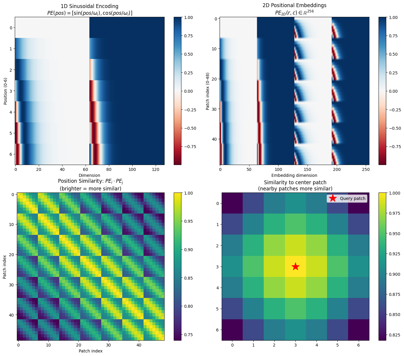


Positional Embedding Properties:
  • Each position gets a unique 256D vector
  • Nearby patches have similar embeddings (high dot product)
  • Distant patches have dissimilar embeddings (low dot product)
  • The model learns to interpret these patterns

Step 3: Self-Attention - The Heart of Transformers¶

Self-attention is what gives transformers their power. Unlike CNNs where each location only sees its local neighborhood, attention lets every token interact with every other token in a single operation.

The Attention Mechanism¶

Given input tokens $X \in \mathbb{R}^{N \times D}$ (N tokens, D dimensions each):

Step 1: Project to Query, Key, Value

Q = XW_Q, \quad K = XW_K, \quad V = XW_V

(7)

where $W_Q, W_K, W_V \in \mathbb{R}^{D \times D}$ are learned projection matrices.

Step 2: Compute attention scores

A = \text{softmax}\left(\frac{QK^T}{\sqrt{D}}\right) \in \mathbb{R}^{N \times N}

(8)

Entry $A_{ij}$ tells us: “How much should token $i$ attend to token $j$ ?”

Step 3: Aggregate values

\text{Output} = AV \in \mathbb{R}^{N \times D}

(9)

Each output token is a weighted combination of all value vectors, with weights from the attention matrix.

Understanding Q, K, V¶

Component	Intuition	Question It Answers
Query (Q)	“What am I looking for?”	What information does this token need?
Key (K)	“What do I contain?”	What information does this token have?
Value (V)	“What do I provide?”	What content should be passed along?

When $Q_i \cdot K_j$ is large, token $i$ strongly attends to token $j$ .

The Scaling Factor $\sqrt{D}$ ¶

Why divide by $\sqrt{D}$ ? Without it:

Dot products $Q_i \cdot K_j$ have variance proportional to $D$
Large values make softmax nearly one-hot
Gradients vanish, training fails

Dividing by $\sqrt{D}$ normalizes the variance to ~1, keeping gradients healthy.

Multi-Head Attention¶

Instead of one attention operation, we run $H$ parallel “heads”:

\text{MultiHead}(X) = \text{Concat}(\text{head}_1, \ldots, \text{head}_H) W_O

(10)

where each head uses dimension $D/H$ . This lets the model attend to different aspects simultaneously - one head might focus on local structure, another on global patterns.

def visualize_attention_mechanism():
    """
    Visualize the self-attention computation step by step.
    """
    N = 7  # 7 tokens (simplified for visualization)
    D = 4  # 4 dimensions
    
    # Create sample input
    np.random.seed(42)
    X = torch.randn(N, D)
    
    # Learned projections (random for illustration)
    W_Q = torch.randn(D, D) * 0.5
    W_K = torch.randn(D, D) * 0.5
    W_V = torch.randn(D, D) * 0.5
    
    # Compute Q, K, V
    Q = X @ W_Q
    K = X @ W_K
    V = X @ W_V
    
    # Compute attention scores
    scores = Q @ K.T / np.sqrt(D)
    attention = torch.softmax(scores, dim=-1)
    
    # Compute output
    output = attention @ V
    
    fig, axes = plt.subplots(2, 4, figsize=(16, 8))
    
    # Row 1: The computation
    vmin, vmax = -2, 2
    
    axes[0, 0].imshow(X.numpy(), cmap='RdBu', vmin=vmin, vmax=vmax)
    axes[0, 0].set_title('Input $X$\n$(N \\times D)$', fontsize=11)
    axes[0, 0].set_xlabel('Dimensions')
    axes[0, 0].set_ylabel('Tokens')
    
    axes[0, 1].imshow(Q.numpy(), cmap='RdBu', vmin=vmin, vmax=vmax)
    axes[0, 1].set_title('Query $Q = XW_Q$\n"What am I looking for?"', fontsize=11)
    axes[0, 1].set_xlabel('Dimensions')
    
    axes[0, 2].imshow(K.numpy(), cmap='RdBu', vmin=vmin, vmax=vmax)
    axes[0, 2].set_title('Key $K = XW_K$\n"What do I contain?"', fontsize=11)
    axes[0, 2].set_xlabel('Dimensions')
    
    axes[0, 3].imshow(V.numpy(), cmap='RdBu', vmin=vmin, vmax=vmax)
    axes[0, 3].set_title('Value $V = XW_V$\n"What do I provide?"', fontsize=11)
    axes[0, 3].set_xlabel('Dimensions')
    
    # Row 2: Attention computation
    axes[1, 0].imshow(scores.numpy(), cmap='RdBu')
    axes[1, 0].set_title('Scores: $QK^T / \\sqrt{D}$', fontsize=11)
    axes[1, 0].set_xlabel('Key token')
    axes[1, 0].set_ylabel('Query token')
    
    im = axes[1, 1].imshow(attention.numpy(), cmap='Reds')
    axes[1, 1].set_title('Attention: $\\text{softmax}(\\cdot)$\n(rows sum to 1)', fontsize=11)
    axes[1, 1].set_xlabel('Key token')
    axes[1, 1].set_ylabel('Query token')
    plt.colorbar(im, ax=axes[1, 1])
    
    axes[1, 2].imshow(output.numpy(), cmap='RdBu', vmin=vmin, vmax=vmax)
    axes[1, 2].set_title('Output: $\\text{Attention} \\times V$', fontsize=11)
    axes[1, 2].set_xlabel('Dimensions')
    axes[1, 2].set_ylabel('Tokens')
    
    # Show attention pattern for one query
    query_idx = 3
    axes[1, 3].bar(range(N), attention[query_idx].numpy())
    axes[1, 3].set_title(f'Token {query_idx} attends to:', fontsize=11)
    axes[1, 3].set_xlabel('Token index')
    axes[1, 3].set_ylabel('Attention weight')
    axes[1, 3].set_ylim(0, 1)
    
    plt.suptitle('Self-Attention: $\\text{Attention}(Q,K,V) = \\text{softmax}(QK^T/\\sqrt{D}) \\cdot V$', fontsize=14)
    plt.tight_layout()
    plt.show()
    
    print(f"\nAttention Properties:")
    print(f"  • Input: {N} tokens × {D} dimensions")
    print(f"  • Attention matrix: {N}×{N} = {N**2} pairwise interactions")
    print(f"  • Each row sums to 1 (probability distribution over keys)")
    print(f"  • Complexity: O(N²D) - quadratic in sequence length")

visualize_attention_mechanism()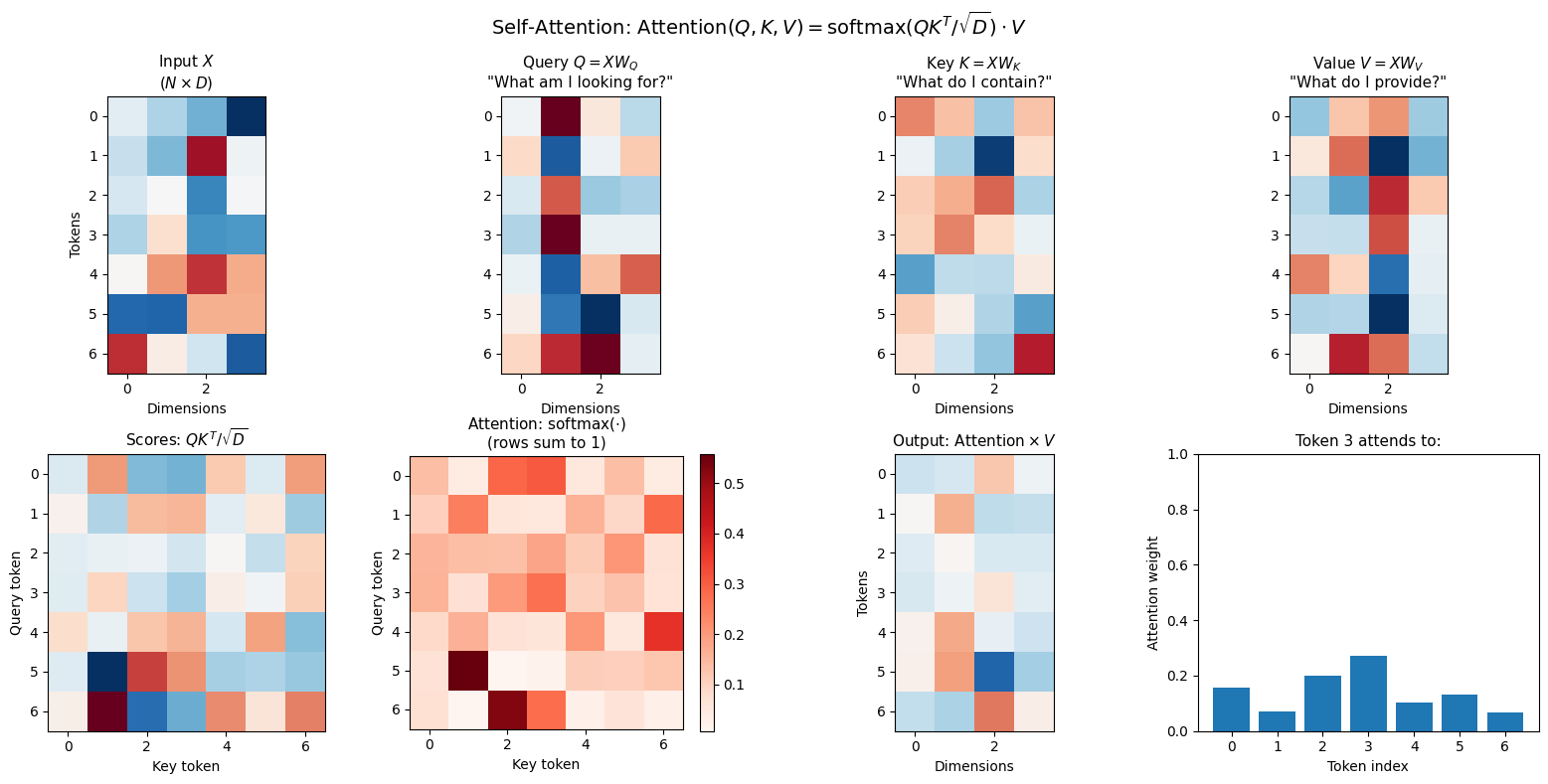


Attention Properties:
  • Input: 7 tokens × 4 dimensions
  • Attention matrix: 7×7 = 49 pairwise interactions
  • Each row sums to 1 (probability distribution over keys)
  • Complexity: O(N²D) - quadratic in sequence length

def visualize_image_attention_patterns():
    """
    Show what attention patterns might look like for image patches.
    """
    grid_size = 7
    N = grid_size ** 2  # 49 patches
    
    fig, axes = plt.subplots(2, 4, figsize=(16, 8))
    
    query_pos = (3, 3)  # Center patch
    query_idx = query_pos[0] * grid_size + query_pos[1]
    
    patterns = [
        ('Uniform', np.ones((grid_size, grid_size)) / N),
        ('Local (Gaussian)', None),
        ('Horizontal', None),
        ('Vertical', None),
        ('Diagonal', None),
        ('Sparse', None),
        ('Learned (example)', None),
        ('Cross', None),
    ]
    
    # Compute patterns
    # Local Gaussian
    local = np.zeros((grid_size, grid_size))
    for i in range(grid_size):
        for j in range(grid_size):
            dist = np.sqrt((i - query_pos[0])**2 + (j - query_pos[1])**2)
            local[i, j] = np.exp(-dist**2 / 2)
    patterns[1] = ('Local (Gaussian)', local / local.sum())
    
    # Horizontal
    horiz = np.zeros((grid_size, grid_size))
    horiz[query_pos[0], :] = 1
    patterns[2] = ('Horizontal', horiz / horiz.sum())
    
    # Vertical
    vert = np.zeros((grid_size, grid_size))
    vert[:, query_pos[1]] = 1
    patterns[3] = ('Vertical', vert / vert.sum())
    
    # Diagonal
    diag = np.zeros((grid_size, grid_size))
    for i in range(grid_size):
        diag[i, i] = 1
        if grid_size - 1 - i >= 0:
            diag[i, grid_size - 1 - i] = 0.5
    patterns[4] = ('Diagonal', diag / diag.sum())
    
    # Sparse (corners + center)
    sparse = np.zeros((grid_size, grid_size))
    sparse[0, 0] = sparse[0, -1] = sparse[-1, 0] = sparse[-1, -1] = 1
    sparse[3, 3] = 2
    patterns[5] = ('Corners + Center', sparse / sparse.sum())
    
    # Learned-like (mixture)
    learned = local + 0.5 * horiz + 0.3 * np.random.rand(grid_size, grid_size)
    patterns[6] = ('Learned (mixed)', learned / learned.sum())
    
    # Cross
    cross = horiz + vert
    patterns[7] = ('Cross', cross / cross.sum())
    
    for idx, (name, pattern) in enumerate(patterns):
        ax = axes[idx // 4, idx % 4]
        im = ax.imshow(pattern, cmap='Reds', vmin=0)
        ax.plot(query_pos[1], query_pos[0], 'b*', markersize=15)
        ax.set_title(name, fontsize=11)
        ax.axis('off')
    
    plt.suptitle('Possible Attention Patterns (star = query patch, red = attention weights)', fontsize=14)
    plt.tight_layout()
    plt.show()
    
    print("\nPatterns the model might learn:")
    print("  • Early layers: Local patterns (like CNN kernels)")
    print("  • Middle layers: Structural patterns (horizontal, vertical strokes)")
    print("  • Late layers: Semantic patterns (attend to digit-specific regions)")
    print("  • The model learns which patterns are useful!")

visualize_image_attention_patterns()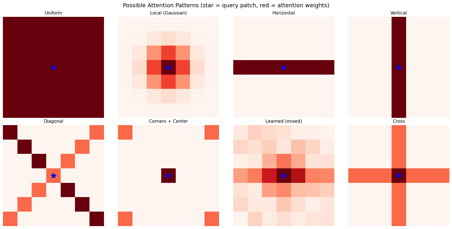


Patterns the model might learn:
  • Early layers: Local patterns (like CNN kernels)
  • Middle layers: Structural patterns (horizontal, vertical strokes)
  • Late layers: Semantic patterns (attend to digit-specific regions)
  • The model learns which patterns are useful!

Step 4: Adaptive Layer Normalization (adaLN)¶

How do we tell the model what timestep we’re at? In the previous notebook, we simply added the timestep embedding to feature maps. DiT uses a more powerful approach: Adaptive Layer Normalization.

Standard Layer Normalization¶

Layer norm normalizes activations and applies a learned affine transform:

\text{LayerNorm}(x) = \gamma \odot \frac{x - \mu}{\sigma} + \beta

(11)

where:

$\mu, \sigma$ = mean and std of $x$ (computed per-sample)
$\gamma, \beta$ = learned scale and shift parameters (same for all inputs)

Adaptive Layer Norm (adaLN)¶

Instead of learned $\gamma, \beta$ , we predict them from the timestep:

[\gamma(t), \beta(t)] = \text{MLP}(\text{time\_embed}(t))

(12)

\text{adaLN}(x, t) = \gamma(t) \odot \frac{x - \mu}{\sigma} + \beta(t)

(13)

Why adaLN Is Powerful¶

Approach	What It Does	Conditioning Strength
Additive $(x + t_{emb})$	Shifts activations	Weak
Concatenation $[x, t_{emb}]$	Separate channels	Medium
adaLN	Scales AND shifts every activation	Strong

adaLN modulates the entire distribution of activations. At each timestep, the model can:

Amplify certain features ( $\gamma > 1$ )
Suppress others ( $\gamma \approx 0$ )
Shift the operating point ( $\beta$ )

Timestep-Dependent Behavior¶

Consider how the task changes with timestep:

$t \approx 1$ (mostly noise): Find large-scale structure, ignore high-frequency details
$t \approx 0$ (mostly data): Refine fine details, preserve structure

adaLN lets the model behave completely differently at different timesteps by controlling which features are active.

from from_noise_to_images.dit import TimestepEmbedding, AdaLN

def visualize_adaln_modulation():
    """
    Show how adaLN parameters vary with timestep.
    """
    embed_dim = 256
    cond_dim = embed_dim * 4
    
    time_embed = TimestepEmbedding(embed_dim, cond_dim)
    adaln = AdaLN(embed_dim, cond_dim)
    
    timesteps = torch.linspace(0, 1, 100)
    
    scales = []
    shifts = []
    
    with torch.no_grad():
        for t in timesteps:
            cond = time_embed(t.unsqueeze(0))
            params = adaln.proj(cond)
            scale, shift = params.chunk(2, dim=-1)
            scales.append(scale.squeeze().numpy())
            shifts.append(shift.squeeze().numpy())
    
    scales = np.array(scales)  # (100, 256)
    shifts = np.array(shifts)
    
    fig, axes = plt.subplots(2, 2, figsize=(14, 10))
    
    # Scale heatmap
    im = axes[0, 0].imshow(scales.T, aspect='auto', cmap='RdBu', 
                           extent=[0, 1, embed_dim, 0], vmin=-1, vmax=1)
    axes[0, 0].set_xlabel('Timestep $t$')
    axes[0, 0].set_ylabel('Dimension')
    axes[0, 0].set_title('Scale $\\gamma(t)$: How much to amplify each dimension')
    plt.colorbar(im, ax=axes[0, 0])
    
    # Shift heatmap
    im = axes[0, 1].imshow(shifts.T, aspect='auto', cmap='RdBu',
                           extent=[0, 1, embed_dim, 0], vmin=-1, vmax=1)
    axes[0, 1].set_xlabel('Timestep $t$')
    axes[0, 1].set_ylabel('Dimension')
    axes[0, 1].set_title('Shift $\\beta(t)$: How much to shift each dimension')
    plt.colorbar(im, ax=axes[0, 1])
    
    # Selected dimensions
    for d in [0, 64, 128, 192]:
        axes[1, 0].plot(timesteps.numpy(), scales[:, d], label=f'dim {d}')
    axes[1, 0].set_xlabel('Timestep $t$')
    axes[1, 0].set_ylabel('Scale $\\gamma$')
    axes[1, 0].set_title('Scale values for selected dimensions')
    axes[1, 0].legend()
    axes[1, 0].grid(True, alpha=0.3)
    
    # Mean ± std
    mean_scale = scales.mean(axis=1)
    std_scale = scales.std(axis=1)
    mean_shift = shifts.mean(axis=1)
    std_shift = shifts.std(axis=1)
    
    axes[1, 1].plot(timesteps.numpy(), mean_scale, 'b-', label='Mean scale', linewidth=2)
    axes[1, 1].fill_between(timesteps.numpy(), mean_scale - std_scale, mean_scale + std_scale, alpha=0.3)
    axes[1, 1].plot(timesteps.numpy(), mean_shift, 'r-', label='Mean shift', linewidth=2)
    axes[1, 1].fill_between(timesteps.numpy(), mean_shift - std_shift, mean_shift + std_shift, alpha=0.3, color='red')
    axes[1, 1].set_xlabel('Timestep $t$')
    axes[1, 1].set_ylabel('Parameter value')
    axes[1, 1].set_title('Mean adaLN parameters (±1 std)')
    axes[1, 1].legend()
    axes[1, 1].grid(True, alpha=0.3)
    
    plt.suptitle('Adaptive Layer Norm: $\\text{adaLN}(x, t) = \\gamma(t) \\odot \\text{Norm}(x) + \\beta(t)$', fontsize=14)
    plt.tight_layout()
    plt.show()
    
    print("\nadaLN Insights:")
    print("  • Each timestep produces different γ and β values")
    print("  • The model can amplify/suppress different features at different t")
    print("  • This is much more expressive than just adding timestep embeddings")
    print(f"  • Formula: output = γ(t) × LayerNorm(x) + β(t)")

visualize_adaln_modulation()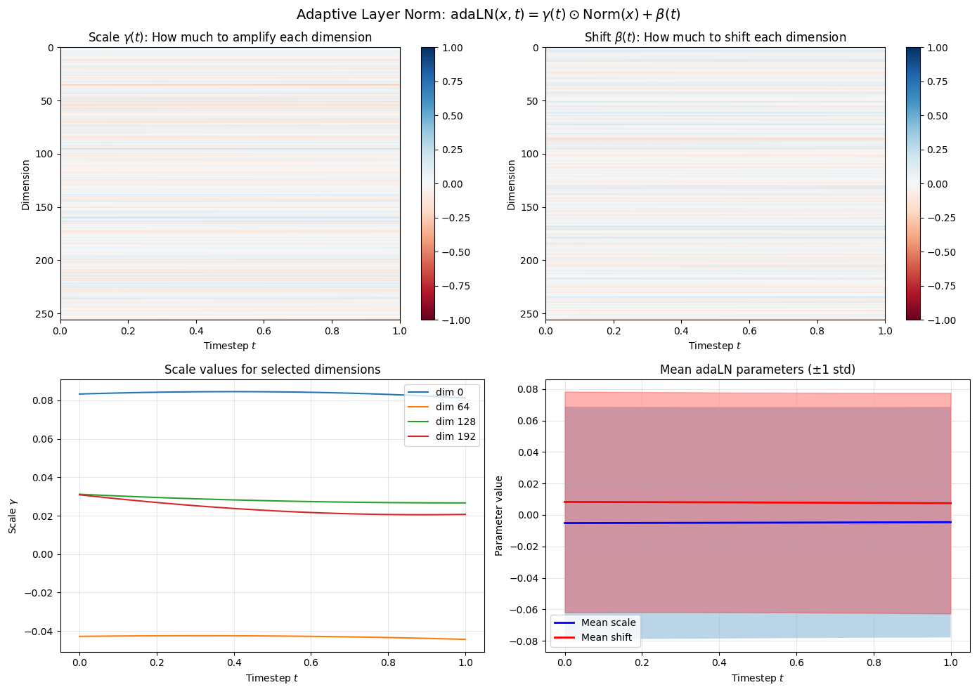


adaLN Insights:
  • Each timestep produces different γ and β values
  • The model can amplify/suppress different features at different t
  • This is much more expressive than just adding timestep embeddings
  • Formula: output = γ(t) × LayerNorm(x) + β(t)

Step 5: The Complete DiT Architecture¶

Now we put all the pieces together. The DiT processes images through:

Forward Pass¶

Patchify: $x \in \mathbb{R}^{H \times W \times C} \rightarrow p \in \mathbb{R}^{N \times (P^2 C)}$
Embed + Position: $z = pE + \text{PE}_{2D} \in \mathbb{R}^{N \times D}$
Timestep Conditioning: $c = \text{MLP}(\text{sinusoidal}(t)) \in \mathbb{R}^{D_c}$
Transformer Blocks (repeat $L$ times):
- $z' = z + \text{Attention}(\text{adaLN}(z, c))$
- $z = z' + \text{MLP}(\text{adaLN}(z', c))$
Unpatchify: $z \in \mathbb{R}^{N \times D} \rightarrow v \in \mathbb{R}^{H \times W \times C}$

DiT Block Structure¶

Input z
   │
   ├───────────────────────────────────┐
   │                                   │ (residual)
   ▼                                   │
adaLN(z, c) ──► Self-Attention ──► + ──┤
                                       │
   ├───────────────────────────────────┘
   │                                   │ (residual)
   ▼                                   │
adaLN(z, c) ──► MLP ──────────────► + ──┘
   │
   ▼
Output z

Computational Complexity¶

Component	Complexity	For MNIST (N=49, D=256)
Self-Attention	$O(N^2 D)$	49² × 256 ≈ 600K ops
MLP	$O(N D^2)$	49 × 256² ≈ 3.2M ops
Per Block	$O(N^2 D + N D^2)$	≈ 3.8M ops
Full Model (6 blocks)		≈ 23M ops

from from_noise_to_images.dit import DiT

# Create DiT model
model = DiT(
    img_size=28,       # MNIST
    patch_size=4,      # 7×7 = 49 patches
    in_channels=1,     # Grayscale
    embed_dim=256,     # Embedding dimension D
    depth=6,           # Number of transformer blocks L
    num_heads=8,       # Attention heads H (256/8 = 32 dim per head)
    mlp_ratio=4.0,     # MLP hidden = 256 × 4 = 1024
).to(device)

num_params = sum(p.numel() for p in model.parameters() if p.requires_grad)
print(f"DiT Parameters: {num_params:,}")
print(f"\nArchitecture:")
print(f"  Patches: 7×7 = 49 (sequence length N)")
print(f"  Embedding: D = 256")
print(f"  Heads: H = 8 (head dim = 256/8 = 32)")
print(f"  MLP hidden: 256 × 4 = 1024")
print(f"  Blocks: L = 6")

# Test forward pass
test_x = torch.randn(4, 1, 28, 28, device=device)
test_t = torch.rand(4, device=device)

with torch.no_grad():
    test_out = model(test_x, test_t)

print(f"\nForward pass:")
print(f"  Input:  {test_x.shape}")
print(f"  Output: {test_out.shape}")
print(f"  Output matches input shape (predicts velocity field)")

DiT Parameters: 12,351,760

Architecture:
  Patches: 7×7 = 49 (sequence length N)
  Embedding: D = 256
  Heads: H = 8 (head dim = 256/8 = 32)
  MLP hidden: 256 × 4 = 1024
  Blocks: L = 6


Forward pass:
  Input:  torch.Size([4, 1, 28, 28])
  Output: torch.Size([4, 1, 28, 28])
  Output matches input shape (predicts velocity field)

# Trace through the model step by step
print("=" * 65)
print("TRACING DiT FORWARD PASS")
print("=" * 65)

x = torch.randn(1, 1, 28, 28, device=device)
t = torch.tensor([0.5], device=device)

print(f"\n1. INPUT")
print(f"   x: {tuple(x.shape)} (image)")
print(f"   t = {t.item():.1f} (timestep)")

with torch.no_grad():
    # Patchify
    patches = model.patch_embed(x)
    print(f"\n2. PATCHIFY")
    print(f"   {x.shape} → {patches.shape}")
    print(f"   (28×28 image → 49 patches × 256 dim)")
    
    # Position embed
    patches_pos = model.pos_embed(patches)
    print(f"\n3. POSITIONAL EMBEDDING")
    print(f"   Add PE: {patches_pos.shape}")
    print(f"   (Each patch now knows its 2D position)")
    
    # Time embed
    cond = model.time_embed(t)
    print(f"\n4. TIMESTEP CONDITIONING")
    print(f"   t={t.item():.1f} → cond: {tuple(cond.shape)}")
    print(f"   (Sinusoidal → MLP → conditioning vector)")
    
    # Transformer blocks
    print(f"\n5. TRANSFORMER BLOCKS (×{len(model.blocks)})")
    print(f"   Each block: adaLN → Attention → adaLN → MLP")
    print(f"   Residual connections preserve information")
    
    # Output
    output = model(x, t)
    print(f"\n6. OUTPUT")
    print(f"   Final norm → Linear → Unpatchify")
    print(f"   {patches.shape} → {output.shape}")
    print(f"   (Predicted velocity field)")

=================================================================
TRACING DiT FORWARD PASS
=================================================================

1. INPUT
   x: (1, 1, 28, 28) (image)
   t = 0.5 (timestep)

2. PATCHIFY
   torch.Size([1, 1, 28, 28]) → torch.Size([1, 49, 256])
   (28×28 image → 49 patches × 256 dim)

3. POSITIONAL EMBEDDING
   Add PE: torch.Size([1, 49, 256])
   (Each patch now knows its 2D position)

4. TIMESTEP CONDITIONING
   t=0.5 → cond: (1, 1024)
   (Sinusoidal → MLP → conditioning vector)

5. TRANSFORMER BLOCKS (×6)
   Each block: adaLN → Attention → adaLN → MLP
   Residual connections preserve information

6. OUTPUT
   Final norm → Linear → Unpatchify
   torch.Size([1, 49, 256]) → torch.Size([1, 1, 28, 28])
   (Predicted velocity field)

Step 6: Training¶

The beauty of flow matching: the training objective is architecture-agnostic:

\mathcal{L} = \mathbb{E}_{x_0, x_1, t}\left[\|v_\theta(x_t, t) - (x_1 - x_0)\|^2\right]

(14)

We can swap U-Net for DiT without changing anything else:

Same forward process: $x_t = (1-t)x_0 + tx_1$
Same velocity target: $v = x_1 - x_0$
Same loss: MSE between predicted and true velocity
Same sampling: Euler integration of the ODE

CNN vs DiT Training¶

Aspect	U-Net (CNN)	DiT
Parameters	~1.8M	~12.4M
Memory	Lower	Higher (attention matrices)
Speed per step	Faster	Slower
Convergence	Quick	Needs more epochs
Scaling	Diminishing returns	Predictable improvement

from from_noise_to_images.train import Trainer

train_loader = DataLoader(
    train_dataset,
    batch_size=128,
    shuffle=True,
    num_workers=0,
    drop_last=True
)

trainer = Trainer(
    model=model,
    dataloader=train_loader,
    lr=1e-4,
    weight_decay=0.01,
    device=device,
)

print("Training DiT with flow matching objective...")
print(f"Loss: L = ||v_theta(x_t, t) - (x_1 - x_0)||^2")
print()

NUM_EPOCHS = 30
losses = trainer.train(num_epochs=NUM_EPOCHS)

Training DiT with flow matching objective...
Loss: L = ||v_theta(x_t, t) - (x_1 - x_0)||^2

Training on cuda
Model parameters: 12,351,760

Epoch 1: avg_loss = 0.8473

Epoch 2: avg_loss = 0.3396

Epoch 3: avg_loss = 0.3046

Epoch 4: avg_loss = 0.2926

Epoch 5: avg_loss = 0.2842

Epoch 6: avg_loss = 0.2790

Epoch 7: avg_loss = 0.2749

Epoch 8: avg_loss = 0.2687

Epoch 9: avg_loss = 0.2586

Epoch 10: avg_loss = 0.2439

Epoch 11: avg_loss = 0.2339

Epoch 12: avg_loss = 0.2265

Epoch 13: avg_loss = 0.2212

Epoch 14: avg_loss = 0.2170

Epoch 15: avg_loss = 0.2143

Epoch 16: avg_loss = 0.2123

Epoch 17: avg_loss = 0.2094

Epoch 18: avg_loss = 0.2079

Epoch 19: avg_loss = 0.2055

Epoch 20: avg_loss = 0.2046

Epoch 21: avg_loss = 0.2026

Epoch 22: avg_loss = 0.2020

Epoch 23: avg_loss = 0.2013

Epoch 24: avg_loss = 0.2005

Epoch 25: avg_loss = 0.1993

Epoch 26: avg_loss = 0.1987

Epoch 27: avg_loss = 0.1968

Epoch 28: avg_loss = 0.1963

Epoch 29: avg_loss = 0.1961

Epoch 30: avg_loss = 0.1951

plt.figure(figsize=(10, 4))
plt.plot(losses, marker='o', markersize=4)
plt.xlabel('Epoch', fontsize=12)
plt.ylabel('MSE Loss', fontsize=12)
plt.title('DiT Training: $\\mathcal{L} = \\|v_\\theta(x_t, t) - v\\|^2$', fontsize=14)
plt.grid(True, alpha=0.3)
plt.show()

print(f"Final loss: {losses[-1]:.4f}")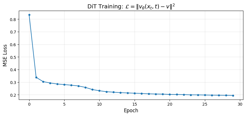

Final loss: 0.1951

Step 7: Generation¶

Generation uses the same ODE as before:

\frac{dx}{dt} = v_\theta(x, t)

(15)

Starting from $x_1 \sim \mathcal{N}(0, I)$ at $t=1$ , integrate backward to $t=0$ :

x_{t-\Delta t} = x_t - \Delta t \cdot v_\theta(x_t, t)

(16)

The DiT’s global attention should produce more coherent samples than the CNN’s local processing.

from from_noise_to_images.sampling import sample

def show_images(images, nrow=8, title=""):
    images = (images + 1) / 2
    images = images.clamp(0, 1)
    grid = torchvision.utils.make_grid(images, nrow=nrow, padding=2)
    plt.figure(figsize=(12, 12 * grid.shape[1] / grid.shape[2]))
    plt.imshow(grid.permute(1, 2, 0).cpu().numpy(), cmap='gray')
    plt.axis('off')
    if title:
        plt.title(title, fontsize=14)
    plt.show()

model.eval()
with torch.no_grad():
    generated, trajectory = sample(
        model=model,
        num_samples=64,
        image_shape=(1, 28, 28),
        num_steps=50,
        device=device,
        return_trajectory=True,
    )

show_images(generated, nrow=8, title="DiT Generated Samples")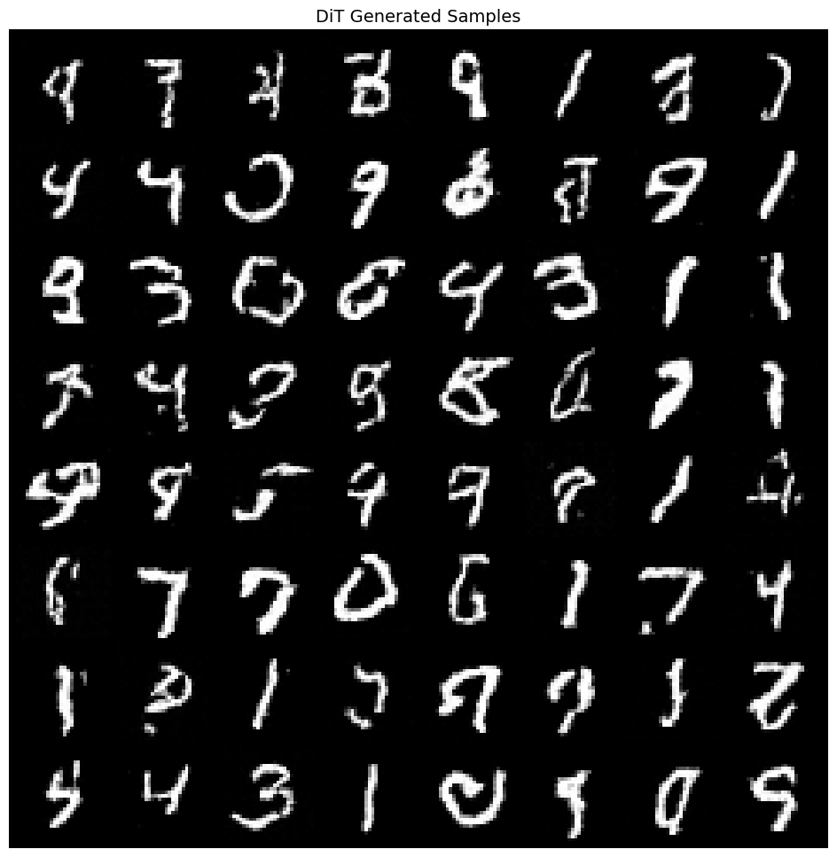

# Visualize generation process
num_to_show = 4
steps_to_show = [0, 5, 10, 20, 30, 40, 50]

fig, axes = plt.subplots(num_to_show, len(steps_to_show), figsize=(14, 8))

for row in range(num_to_show):
    for col, step_idx in enumerate(steps_to_show):
        img = (trajectory[step_idx][row, 0] + 1) / 2
        axes[row, col].imshow(img.cpu().numpy(), cmap='gray')
        axes[row, col].axis('off')
        if row == 0:
            t_val = 1.0 - step_idx / 50
            axes[row, col].set_title(f'$t={t_val:.2f}$')

plt.suptitle('DiT Generation: Solving $dx/dt = v_\\theta(x,t)$ from $t=1$ to $t=0$', fontsize=14)
plt.tight_layout()
plt.show()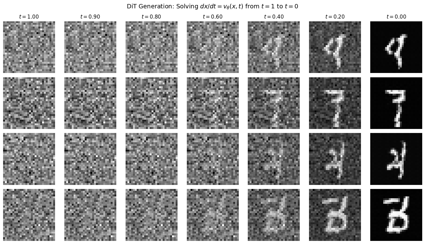

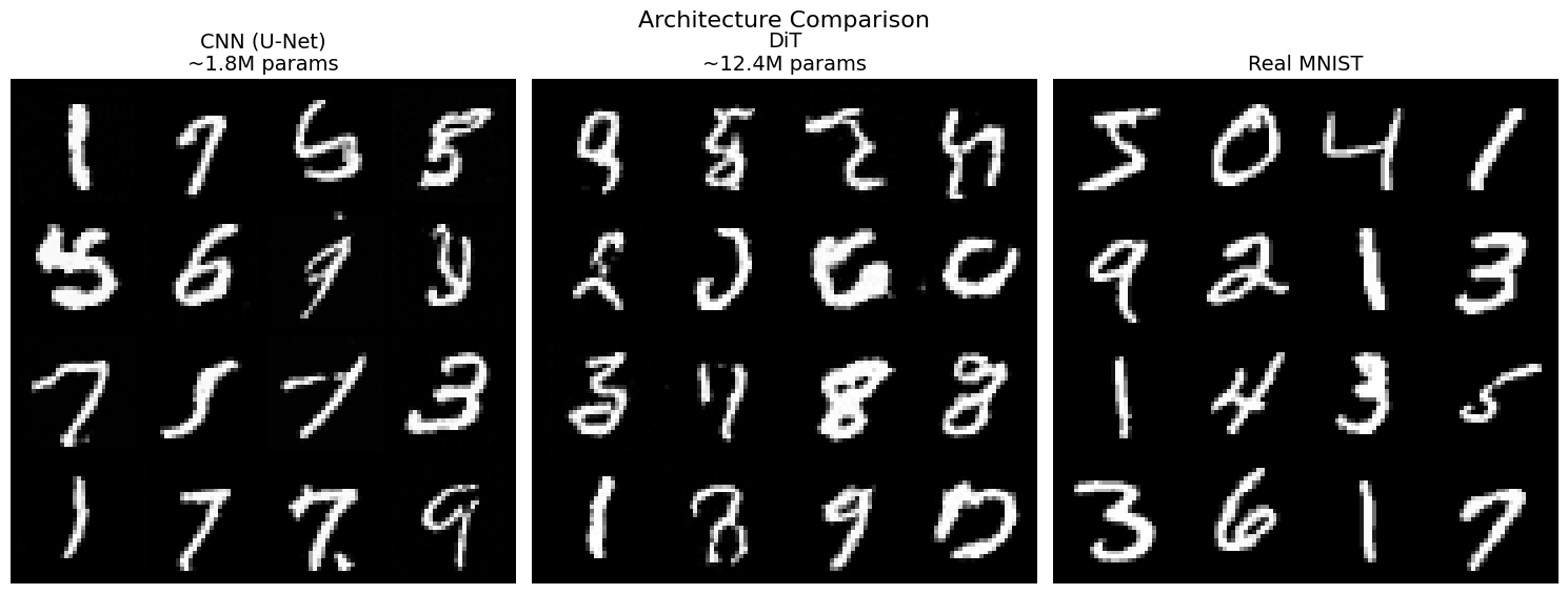
Step 8: CNN vs DiT Comparison¶

Let’s compare the two architectures side by side:

Architecture	Parameters	Receptive Field	Conditioning
U-Net (CNN)	~1.8M	Local → Global	Additive
DiT	~12.4M	Global (layer 1)	adaLN (multiplicative)

import os
from from_noise_to_images.models import SimpleUNet

# Load or train CNN
cnn_model = SimpleUNet(in_channels=1, model_channels=64, time_emb_dim=128).to(device)

if os.path.exists("phase1_model.pt"):
    print("Loading CNN from phase1_model.pt...")
    checkpoint = torch.load("phase1_model.pt", map_location=device)
    cnn_model.load_state_dict(checkpoint["model_state_dict"])
else:
    print("Training CNN for comparison...")
    cnn_trainer = Trainer(model=cnn_model, dataloader=train_loader, lr=1e-4, device=device)
    cnn_trainer.train(num_epochs=NUM_EPOCHS)

# Generate from both
model.eval()
cnn_model.eval()

with torch.no_grad():
    dit_samples = sample(model, 16, (1, 28, 28), 50, device)
    cnn_samples = sample(cnn_model, 16, (1, 28, 28), 50, device)

real_samples = torch.stack([train_dataset[i][0] for i in range(16)])

# Compare
fig, axes = plt.subplots(1, 3, figsize=(15, 6))

for ax, samples, title in [
    (axes[0], cnn_samples, 'CNN (U-Net)\n~1.8M params'),
    (axes[1], dit_samples, 'DiT\n~12.4M params'),
    (axes[2], real_samples, 'Real MNIST'),
]:
    grid = torchvision.utils.make_grid((samples + 1) / 2, nrow=4, padding=2)
    ax.imshow(grid.permute(1, 2, 0).cpu().numpy(), cmap='gray')
    ax.set_title(title, fontsize=14)
    ax.axis('off')

plt.suptitle('Architecture Comparison', fontsize=16)
plt.tight_layout()
plt.show()

Loading CNN from phase1_model.pt...

Clipping input data to the valid range for imshow with RGB data ([0..1] for floats or [0..255] for integers). Got range [-0.014467537..1.0167499].

Clipping input data to the valid range for imshow with RGB data ([0..1] for floats or [0..255] for integers). Got range [-0.058273673..1.057965].

# Save model for next notebook
trainer.save_checkpoint("phase2_dit.pt")
print("Model saved to phase2_dit.pt")

Model saved to phase2_dit.pt

Summary: What We Built¶

We replaced the CNN with a Diffusion Transformer that processes images through:

The Pipeline¶

Step	Operation	Result
Patchify	$x \in \mathbb{R}^{28 \times 28}$ → patches	$z \in \mathbb{R}^{49 \times 256}$
Position	Add 2D sinusoidal encoding	Spatial awareness
Attention	$\text{softmax}(QK^T/\sqrt{d})V$	Global interactions
adaLN	$\gamma(t) \cdot \text{Norm}(x) + \beta(t)$	Timestep conditioning
Unpatchify	$z \in \mathbb{R}^{49 \times 256}$ → image	$v \in \mathbb{R}^{28 \times 28}$

Key Concepts¶

Concept	Formula	Purpose
Patchify	$z = xE + PE$	Image to sequence
Attention	$\text{softmax}(QK^T/\sqrt{d})V$	Global interactions
adaLN	$\gamma(t) \odot \text{Norm}(x) + \beta(t)$	Timestep conditioning
Training	$\|v_\theta(x_t,t) - v\|^2$	Learn velocity field

Why DiT Matters¶

Global from layer 1: Every patch sees every other patch immediately
Scaling laws: Predictable improvement with more compute
Strong conditioning: adaLN modulates all activations per-timestep
Architectural simplicity: Just stack identical blocks

What’s Next¶

In the next notebook, we add class conditioning to control generation:

Class embeddings combined with timestep
Classifier-Free Guidance (CFG)
“Generate a 7” → produces a 7!