Flow Matching: Learning to Transform Noise into Data

Every image you’ve ever seen from Stable Diffusion, Midjourney, or DALL-E started as pure random noise. A generative model learned to transform that noise into coherent images. In this notebook, we’ll build one from scratch.

We’ll use flow matching - a beautifully simple approach that has become the foundation for state-of-the-art image generation. By the end, you’ll have a model that can generate handwritten digits from nothing but Gaussian noise.

The Problem We’re Solving¶

Here’s the setup:

We have training data $x \sim p_{\text{data}}(x)$ (real MNIST digits)
We want to sample new images from $p_{\text{data}}$
But we don’t know $p_{\text{data}}$ explicitly - we only have examples

The strategy: learn a transformation from a simple distribution (Gaussian noise) to our complex data distribution. If we can learn this transformation, we can generate new samples by:

Sample noise $z \sim \mathcal{N}(0, I)$
Apply our learned transformation
Out comes a realistic image!

Why Flow Matching?¶

Several approaches exist for generative modeling:

Approach	Core Idea	Challenge
GANs	Generator fools discriminator	Training instability, mode collapse
VAEs	Encode/decode through latent space	Blurry outputs, approximate posteriors
DDPM	Gradually denoise over many steps	Stochastic, slow sampling, complex math
Flow Matching	Learn straight paths from noise to data	Simple, fast, deterministic

Flow matching has become the preferred choice because:

Simpler mathematics - no stochastic differential equations required
Faster sampling - straight paths require fewer integration steps
Same training objective works for any architecture
State-of-the-art results - used in Stable Diffusion 3, Flux, and more

The Mathematical Framework¶

Probability Paths: The Core Intuition¶

Imagine two probability distributions:

$p_0$ : The data distribution (complex, what we want to sample from)
$p_1$ : A simple distribution (standard Gaussian, easy to sample)

Flow matching constructs a continuous path of distributions $p_t$ that smoothly transitions between them:

p_0 \xrightarrow{t=0 \to 1} p_1

(1)

The key insight: if we can describe how individual samples move along this path, we can:

Train: Learn the “velocity” of samples at each point
Generate: Start from $p_1$ (noise) and follow velocities backward to $p_0$ (data)

Linear Interpolation: The Simplest Path¶

How do we connect a data point $x_0$ to a noise sample $x_1$ ? The simplest choice is a straight line:

x_t = (1-t) \cdot x_0 + t \cdot x_1

(2)

Let’s verify this gives us what we want:

$t$	$x_t$	Description
0	$(1-0)x_0 + 0 \cdot x_1 = x_0$	Pure data
0.5	$0.5 \cdot x_0 + 0.5 \cdot x_1$	Half data, half noise
1	$0 \cdot x_0 + 1 \cdot x_1 = x_1$	Pure noise

Perfect. As $t$ goes from 0 to 1, we trace a straight line from the data point to the noise sample.

(This linear path is sometimes called rectified flow or optimal transport flow, because straight lines are the shortest paths between points.)

The Velocity Field¶

The velocity tells us how $x_t$ changes as $t$ increases. Let’s derive it:

v = \frac{dx_t}{dt} = \frac{d}{dt}\left[(1-t) \cdot x_0 + t \cdot x_1\right]

(3)

Taking the derivative term by term:

v = \frac{d}{dt}[(1-t)] \cdot x_0 + \frac{d}{dt}[t] \cdot x_1 = -x_0 + x_1 = x_1 - x_0

(4)

This result is remarkable: the velocity is constant! It doesn’t depend on $t$ at all.

Why does this matter?

Each sample travels in a perfectly straight line
The velocity is simply the direction from data to noise
No curved paths, no acceleration - just constant motion

The Neural Network’s Job¶

We train a neural network $v_\theta(x_t, t)$ to predict the velocity given:

$x_t$ : The current “noised” sample (a blend of data and noise)
$t$ : The current timestep

The training loss is straightforward MSE:

\mathcal{L} = \mathbb{E}_{x_0 \sim p_{\text{data}}, \, x_1 \sim \mathcal{N}(0,I), \, t \sim U[0,1]}\left[\|v_\theta(x_t, t) - (x_1 - x_0)\|^2\right]

(5)

In words: sample data, sample noise, sample timestep, compute the interpolation $x_t$ , predict velocity, compare to true velocity $x_1 - x_0$ .

Generating Samples: Solving the ODE¶

Once trained, generation is an ordinary differential equation (ODE):

\frac{dx_t}{dt} = v_\theta(x_t, t)

(6)

We start at $t=1$ with pure noise $x_1 \sim \mathcal{N}(0, I)$ and integrate backward to $t=0$ :

x_0 = x_1 - \int_1^0 v_\theta(x_t, t) \, dt = x_1 + \int_0^1 v_\theta(x_t, t) \, dt

(7)

In practice, we use Euler integration:

x_{t-\Delta t} = x_t - \Delta t \cdot v_\theta(x_t, t)

(8)

Starting at $t=1$ , we take small steps backward until we reach $t=0$ .

Key Equations at a Glance¶

Concept	Equation	What It Does
Interpolation	$x_t = (1-t)x_0 + tx_1$	Creates path from data to noise
Velocity	$v = x_1 - x_0$	Direction of travel (constant!)
Training Loss	$\mathcal{L} = \|v_\theta(x_t, t) - v\|^2$	MSE between predicted and true velocity
Sampling ODE	$\frac{dx}{dt} = v_\theta(x, t)$	Defines the generation dynamics
Euler Step	$x_{t-\Delta t} = x_t - \Delta t \cdot v_\theta$	Discrete approximation for sampling

Now let’s implement this.

import torch
import torch.nn as nn
import torchvision
import torchvision.transforms as transforms
from torch.utils.data import DataLoader
import matplotlib.pyplot as plt
import numpy as np

# Auto-reload modules during development
%load_ext autoreload
%autoreload 2

# Set up device
if torch.backends.mps.is_available():
    device = torch.device("mps")
elif torch.cuda.is_available():
    device = torch.device("cuda")
else:
    device = torch.device("cpu")
print(f"Using device: {device}")

Using device: cuda

Step 1: The Data Distribution¶

We’ll use MNIST - 28×28 grayscale handwritten digits. It’s ideal for learning:

Small images (784 pixels) = fast training
Simple enough to verify visually
Complex enough to be interesting (10 digit classes, varying styles)

Important preprocessing: We normalize pixels to $[-1, 1]$ instead of $[0, 1]$ . Why? Our noise distribution $\mathcal{N}(0, I)$ is centered at zero with values typically in $[-3, 3]$ . Centering our data similarly makes the interpolation path more balanced.

# Transform: convert to tensor and normalize to [-1, 1]
transform = transforms.Compose([
    transforms.ToTensor(),
    transforms.Normalize((0.5,), (0.5,))  # Maps [0,1] to [-1,1]
])

# Download and load MNIST
train_dataset = torchvision.datasets.MNIST(
    root="./data",
    train=True,
    download=True,
    transform=transform
)

train_loader = DataLoader(
    train_dataset,
    batch_size=128,
    shuffle=True,
    num_workers=0,  # Set to 0 for MPS compatibility
    drop_last=True
)

print(f"Dataset size: {len(train_dataset):,} images")
print(f"Batches per epoch: {len(train_loader)}")
print(f"Image shape: {train_dataset[0][0].shape}")
print(f"Pixel range: [{train_dataset[0][0].min():.1f}, {train_dataset[0][0].max():.1f}]")

Dataset size: 60,000 images
Batches per epoch: 468
Image shape: torch.Size([1, 28, 28])
Pixel range: [-1.0, 1.0]

# Visualize some training samples
def show_images(images, nrow=8, title=""):
    """Display a grid of images."""
    # Denormalize from [-1, 1] to [0, 1]
    images = (images + 1) / 2
    images = images.clamp(0, 1)
    
    grid = torchvision.utils.make_grid(images, nrow=nrow, padding=2)
    plt.figure(figsize=(12, 12 * grid.shape[1] / grid.shape[2]))
    plt.imshow(grid.permute(1, 2, 0).cpu().numpy(), cmap='gray')
    plt.axis('off')
    if title:
        plt.title(title, fontsize=14)
    plt.show()

# Get a batch and visualize
sample_batch, _ = next(iter(train_loader))
show_images(sample_batch[:32], title="Training samples from $p_{data}$ (MNIST digits)")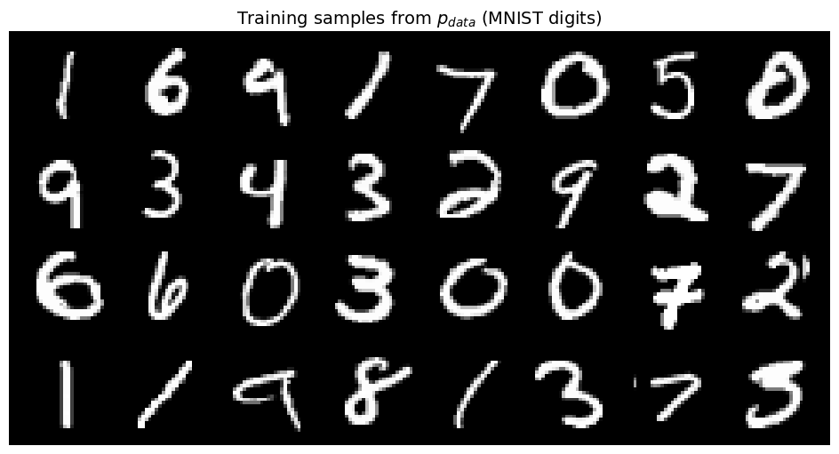

Step 2: The Forward Process (Data → Noise)¶

Let’s implement and visualize the interpolation path from data to noise.

The Interpolation Formula¶

For a data point $x_0$ and noise sample $x_1 \sim \mathcal{N}(0, I)$ :

x_t = (1-t) \cdot x_0 + t \cdot x_1

(9)

Geometric Picture¶

Think of each image as a point in 784-dimensional space (one dimension per pixel):

$x_0$ lives on the “data manifold” - the region where realistic digits reside
$x_1$ is a random point in space (Gaussian noise spreads throughout)
$x_t$ traces a straight line between them

During training, we’ll show the network samples $x_t$ at random timesteps and ask it to predict which direction leads toward noise.

from from_noise_to_images.flow import FlowMatching

flow = FlowMatching()

# Take one image and show its path to noise
x_0 = sample_batch[0:1]  # Shape: (1, 1, 28, 28)
x_1 = torch.randn_like(x_0)  # Sample noise ~ N(0, I)

# Show interpolation at different timesteps
timesteps = [0.0, 0.2, 0.4, 0.6, 0.8, 1.0]
interpolated = []

for t in timesteps:
    t_tensor = torch.tensor([t])
    x_t, velocity = flow.forward_process(x_0, x_1, t_tensor)
    interpolated.append(x_t)

# Visualize
fig, axes = plt.subplots(1, len(timesteps), figsize=(15, 3))
for i, (ax, t) in enumerate(zip(axes, timesteps)):
    img = (interpolated[i][0, 0] + 1) / 2  # Denormalize
    ax.imshow(img.numpy(), cmap='gray')
    ax.set_title(f'$t = {t}$', fontsize=12)
    ax.axis('off')
    
    # Add equation annotation
    if t == 0.0:
        ax.set_xlabel('$x_0$ (data)', fontsize=10)
    elif t == 1.0:
        ax.set_xlabel('$x_1$ (noise)', fontsize=10)
    elif t == 0.5:
        ax.set_xlabel('$0.5 x_0 + 0.5 x_1$', fontsize=10)

plt.suptitle('Forward Process: $x_t = (1-t) x_0 + t x_1$', fontsize=14)
plt.tight_layout()
plt.show()

print("\nWatch how the digit structure gradually dissolves into noise.")
print("Our model will learn to reverse this process.")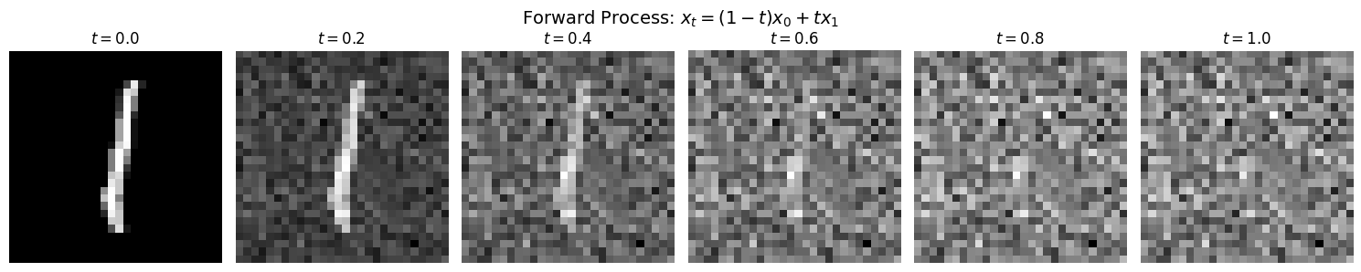


Watch how the digit structure gradually dissolves into noise.
Our model will learn to reverse this process.

Step 3: Understanding the Velocity Field¶

Deriving the Velocity¶

The velocity is the time derivative of our interpolation:

v = \frac{dx_t}{dt} = \frac{d}{dt}\left[(1-t) x_0 + t x_1\right]

(10)

Let’s work through this carefully:

v = \frac{d}{dt}[(1-t)] \cdot x_0 + (1-t) \cdot \frac{d}{dt}[x_0] + \frac{d}{dt}[t] \cdot x_1 + t \cdot \frac{d}{dt}[x_1]

(11)

Since $x_0$ and $x_1$ are constants (they don’t depend on $t$ ):

v = (-1) \cdot x_0 + 0 + (1) \cdot x_1 + 0 = x_1 - x_0

(12)

The Key Property: Constant Velocity¶

Notice that $v = x_1 - x_0$ has no $t$ in it. This means:

Property	Implication
Velocity is constant	Samples travel in straight lines
Same velocity at all $t$	No acceleration, no curved paths
$v = x_1 - x_0$	Velocity encodes the displacement from data to noise

What Does the Velocity Look Like?¶

Since $v = x_1 - x_0$ (pixel-wise subtraction):

Where noise is brighter than data ( $x_1 > x_0$ ): positive velocity (pixel brightens)
Where noise is darker than data ( $x_1 < x_0$ ): negative velocity (pixel darkens)
The velocity is essentially a “difference image”

# Compute and visualize the velocity field for a single example
t_tensor = torch.tensor([0.5])  # Timestep doesn't matter for velocity!
x_t, velocity = flow.forward_process(x_0, x_1, t_tensor)

fig, axes = plt.subplots(1, 4, figsize=(16, 4))

# Data point x_0
axes[0].imshow((x_0[0, 0] + 1) / 2, cmap='gray')
axes[0].set_title('$x_0$ (data)', fontsize=12)
axes[0].axis('off')

# Noise point x_1
axes[1].imshow((x_1[0, 0] + 1) / 2, cmap='gray')
axes[1].set_title('$x_1$ (noise)', fontsize=12)
axes[1].axis('off')

# Velocity v = x_1 - x_0
v_display = velocity[0, 0].numpy()
im = axes[2].imshow(v_display, cmap='RdBu', vmin=-2, vmax=2)
axes[2].set_title('$v = x_1 - x_0$ (velocity)', fontsize=12)
axes[2].axis('off')
plt.colorbar(im, ax=axes[2], fraction=0.046)

# Interpolated sample at t=0.5
axes[3].imshow((x_t[0, 0] + 1) / 2, cmap='gray')
axes[3].set_title('$x_{0.5}$ (midpoint)', fontsize=12)
axes[3].axis('off')

plt.suptitle('The Velocity Field: Direction from Data to Noise', fontsize=14)
plt.tight_layout()
plt.show()

print("\nInterpreting the velocity:")
print("• Red: noise brighter than data → positive velocity")
print("• Blue: noise darker than data → negative velocity")
print("• White: similar values → near-zero velocity")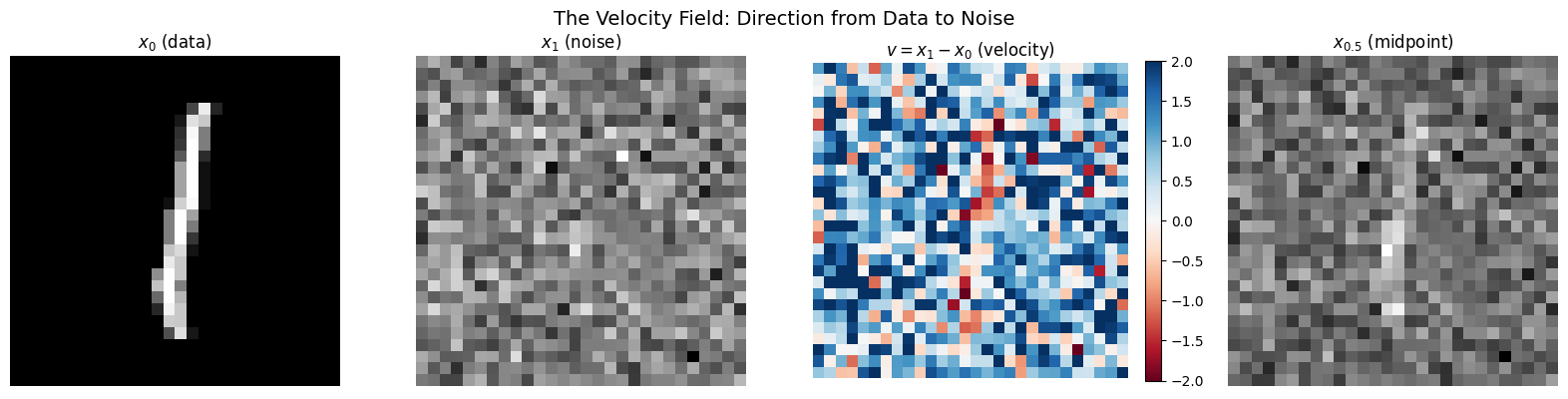


Interpreting the velocity:
• Red: noise brighter than data → positive velocity
• Blue: noise darker than data → negative velocity
• White: similar values → near-zero velocity

# Verify: velocity is constant at all timesteps
print("Verifying that velocity is constant along the path...")
print()

for t in [0.0, 0.25, 0.5, 0.75, 1.0]:
    t_tensor = torch.tensor([t])
    _, v = flow.forward_process(x_0, x_1, t_tensor)
    v_norm = torch.norm(v).item()
    print(f"t = {t:.2f}: ||v|| = {v_norm:.4f}")

print()
print("✓ Velocity norm is identical at all timesteps!")
print("  This confirms v = x₁ - x₀ doesn't depend on t.")

Verifying that velocity is constant along the path...

t = 0.00: ||v|| = 38.0034
t = 0.25: ||v|| = 38.0034
t = 0.50: ||v|| = 38.0034
t = 0.75: ||v|| = 38.0034
t = 1.00: ||v|| = 38.0034

✓ Velocity norm is identical at all timesteps!
  This confirms v = x₁ - x₀ doesn't depend on t.

Step 4: The Neural Network Architecture¶

We need a neural network $v_\theta(x_t, t)$ that:

Input: Noised image $x_t$ (28×28×1) + timestep $t$ (scalar)
Output: Predicted velocity $\hat{v}$ (28×28×1, same shape as input)

U-Net: The Classic Choice¶

We use a U-Net, a proven architecture for image-to-image tasks:

Input (28×28) ──┐                      ┌── Output (28×28)
                ▼                      ▲
            [Encoder]              [Decoder]
                │                      │
           downsample              upsample
                │                      │
                ▼                      ▲
            (14×14)    ──────────>  (14×14)  ← skip connection
                │                      │
           downsample              upsample
                │                      │
                ▼                      ▲
             (7×7)     ──────────>   (7×7)   ← skip connection
                │                      │
                └─────> bottleneck ────┘

Why U-Net? The skip connections let fine-grained details flow directly to the output, while the bottleneck captures global context.

Timestep Conditioning¶

The network needs to know the current timestep $t$ . A scalar isn’t expressive enough, so we use sinusoidal positional encoding (from the Transformer paper):

\text{emb}(t) = \left[\sin(\omega_1 t), \cos(\omega_1 t), \sin(\omega_2 t), \cos(\omega_2 t), \ldots\right]

(13)

where $\omega_i = 10000^{-2i/d}$ spans multiple frequencies. This rich embedding is projected and added to the network’s feature maps at each layer.

from from_noise_to_images.models import SimpleUNet

model = SimpleUNet(
    in_channels=1,       # Grayscale images
    model_channels=64,   # Base channel count (doubled at each level)
    time_emb_dim=128,    # Timestep embedding dimension
).to(device)

# Count parameters
num_params = sum(p.numel() for p in model.parameters() if p.requires_grad)
print(f"Model parameters: {num_params:,}")
print(f"\nThis is relatively small - larger models give better quality.")

# Test forward pass
test_x = torch.randn(4, 1, 28, 28, device=device)
test_t = torch.rand(4, device=device)

with torch.no_grad():
    test_out = model(test_x, test_t)

print(f"\nForward pass test:")
print(f"  Input shape:  {test_x.shape}  (batch, channels, height, width)")
print(f"  Timestep:     {test_t.shape}  (batch,)")
print(f"  Output shape: {test_out.shape}  (same as input - velocity at each pixel)")

Model parameters: 1,837,185

This is relatively small - larger models give better quality.


Forward pass test:
  Input shape:  torch.Size([4, 1, 28, 28])  (batch, channels, height, width)
  Timestep:     torch.Size([4])  (batch,)
  Output shape: torch.Size([4, 1, 28, 28])  (same as input - velocity at each pixel)

Step 5: Training the Velocity Predictor¶

The Training Loop¶

For each training step:

Sample data: $x_0 \sim p_{\text{data}}$ (batch of real digits)
Sample noise: $x_1 \sim \mathcal{N}(0, I)$ (same shape as $x_0$ )
Sample timestep: $t \sim \text{Uniform}[0, 1]$
Compute interpolation: $x_t = (1-t) x_0 + t x_1$
Compute true velocity: $v = x_1 - x_0$
Predict velocity: $\hat{v} = v_\theta(x_t, t)$
Compute loss: $\mathcal{L} = \|\hat{v} - v\|^2$ (MSE)
Update weights: Backprop and optimizer step

Why Does This Work?¶

The model sees many triplets $(x_t, t) \to v$ :

Different data points $x_0$
Different noise samples $x_1$
Different timesteps $t$

It learns patterns like:

“At $t \approx 1$ (mostly noise), velocities point toward structure”
“At $t \approx 0$ (mostly data), velocities are small adjustments”

The key insight: by learning the conditional expectation of velocity given $x_t$ and $t$ , the model implicitly learns the marginal distribution $p_t$ at each timestep.

(There’s deep theory here connecting to optimal transport and continuity equations, but the practical algorithm is beautifully simple.)

from from_noise_to_images.train import Trainer

# Create trainer
trainer = Trainer(
    model=model,
    dataloader=train_loader,
    lr=1e-4,           # Learning rate
    weight_decay=0.01, # Regularization
    device=device,
)

# Train
NUM_EPOCHS = 30  # Increase to 50+ for better quality

print("Training the velocity prediction network...")
print(f"Epochs: {NUM_EPOCHS}")
print(f"Batch size: {train_loader.batch_size}")
print(f"Batches per epoch: {len(train_loader)}")
print()

losses = trainer.train(num_epochs=NUM_EPOCHS)

Training the velocity prediction network...
Epochs: 30
Batch size: 128
Batches per epoch: 468

Training on cuda
Model parameters: 1,837,185

Loading...

Epoch 1: avg_loss = 0.3532

Loading...

Epoch 2: avg_loss = 0.2299

Loading...

Epoch 3: avg_loss = 0.2115

Loading...

Epoch 4: avg_loss = 0.2036

Loading...

Epoch 5: avg_loss = 0.1984

Loading...

Epoch 6: avg_loss = 0.1948

Loading...

Epoch 7: avg_loss = 0.1926

Loading...

Epoch 8: avg_loss = 0.1890

Loading...

Epoch 9: avg_loss = 0.1872

Loading...

Epoch 10: avg_loss = 0.1864

Loading...

Epoch 11: avg_loss = 0.1843

Loading...

Epoch 12: avg_loss = 0.1833

Loading...

Epoch 13: avg_loss = 0.1827

Loading...

Epoch 14: avg_loss = 0.1813

Loading...

Epoch 15: avg_loss = 0.1802

Loading...

Epoch 16: avg_loss = 0.1791

Loading...

Epoch 17: avg_loss = 0.1790

Loading...

Epoch 18: avg_loss = 0.1780

Loading...

Epoch 19: avg_loss = 0.1770

Loading...

Epoch 20: avg_loss = 0.1783

Loading...

Epoch 21: avg_loss = 0.1769

Loading...

Epoch 22: avg_loss = 0.1770

Loading...

Epoch 23: avg_loss = 0.1759

Loading...

Epoch 24: avg_loss = 0.1752

Loading...

Epoch 25: avg_loss = 0.1747

Loading...

Epoch 26: avg_loss = 0.1754

Loading...

Epoch 27: avg_loss = 0.1744

Loading...

Epoch 28: avg_loss = 0.1739

Loading...

Epoch 29: avg_loss = 0.1737

Loading...

Epoch 30: avg_loss = 0.1739

# Plot training loss
plt.figure(figsize=(10, 4))
plt.plot(losses, marker='o', markersize=4)
plt.xlabel('Epoch', fontsize=12)
plt.ylabel('MSE Loss', fontsize=12)
plt.title(r'Training Loss: $\mathcal{L} = \|v_\theta(x_t, t) - (x_1 - x_0)\|^2$', fontsize=14)
plt.grid(True, alpha=0.3)
plt.show()

print(f"Final loss: {losses[-1]:.4f}")
print("\nLower loss = better velocity predictions = better generation.")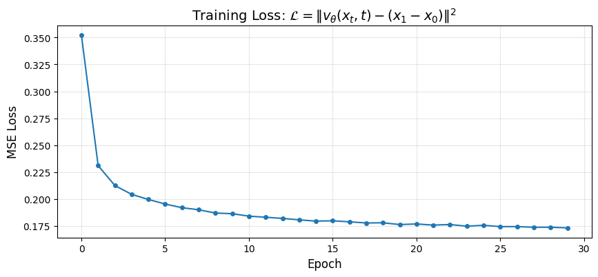

Final loss: 0.1739

Lower loss = better velocity predictions = better generation.

Step 6: Generating New Images¶

Now for the exciting part - using our trained model to generate new digits from scratch!

The Sampling ODE¶

We solve:

\frac{dx}{dt} = v_\theta(x, t)

(14)

Starting point: $x_1 \sim \mathcal{N}(0, I)$ (pure random noise at $t=1$ )

Goal: Integrate backward to $t=0$ to get a sample from $p_{\text{data}}$

Euler Integration¶

We discretize time into $N$ steps with $\Delta t = 1/N$ :

x_{t - \Delta t} = x_t - \Delta t \cdot v_\theta(x_t, t)

(15)

At each step:

Ask the model: “What’s the velocity at this point?”
Move in the opposite direction (we’re going backward in time)
Repeat until we reach $t=0$

Why Backward?¶

During training, velocities point from data to noise ( $x_1 - x_0$ ).

During sampling, we want the reverse - from noise to data - so we:

Start at $t=1$ (noise)
Subtract the velocity (opposite direction)
End at $t=0$ (data)

from from_noise_to_images.sampling import sample

# Generate samples
model.eval()

print("Generating 64 new digits from random noise...")
print("(Starting at t=1, integrating backward to t=0)")
print()

with torch.no_grad():
    generated, trajectory = sample(
        model=model,
        num_samples=64,
        image_shape=(1, 28, 28),
        num_steps=50,      # Number of Euler steps
        device=device,
        return_trajectory=True,
    )

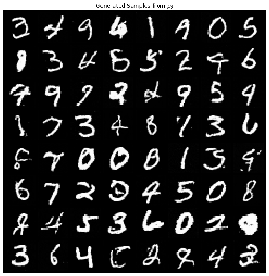
show_images(generated, nrow=8, title="Generated Samples from $p_{\\theta}$")

Generating 64 new digits from random noise...
(Starting at t=1, integrating backward to t=0)

Loading...

Step 7: Visualizing the Generation Process¶

Let’s watch how noise transforms into digits step by step.

This shows the ODE integration in action:

$t=1.00$ : Pure noise $x_1 \sim \mathcal{N}(0, I)$
$t \to 0$ : Following $-v_\theta(x, t)$ backward
$t=0.00$ : Generated digit

# Show the trajectory for a few samples
num_to_show = 4
steps_to_show = [0, 5, 10, 20, 30, 40, 50]  # Which steps to visualize

fig, axes = plt.subplots(num_to_show, len(steps_to_show), figsize=(14, 8))

for row in range(num_to_show):
    for col, step_idx in enumerate(steps_to_show):
        img = trajectory[step_idx][row, 0]
        img = (img + 1) / 2  # Denormalize
        axes[row, col].imshow(img.cpu().numpy(), cmap='gray')
        axes[row, col].axis('off')
        if row == 0:
            t_val = 1.0 - step_idx / 50
            axes[row, col].set_title(f'$t={t_val:.2f}$', fontsize=11)

plt.suptitle('Generation Process: Solving $dx/dt = v_\\theta(x, t)$ backward from $t=1$ to $t=0$', fontsize=14)
plt.tight_layout()
plt.show()

print("\nWatch how structure emerges:")
print("• t≈1.0: Random noise (no discernible pattern)")
print("• t≈0.6: Large-scale structure appears (rough digit shape)")
print("• t≈0.3: Details emerge (strokes, curves)")
print("• t=0.0: Final digit")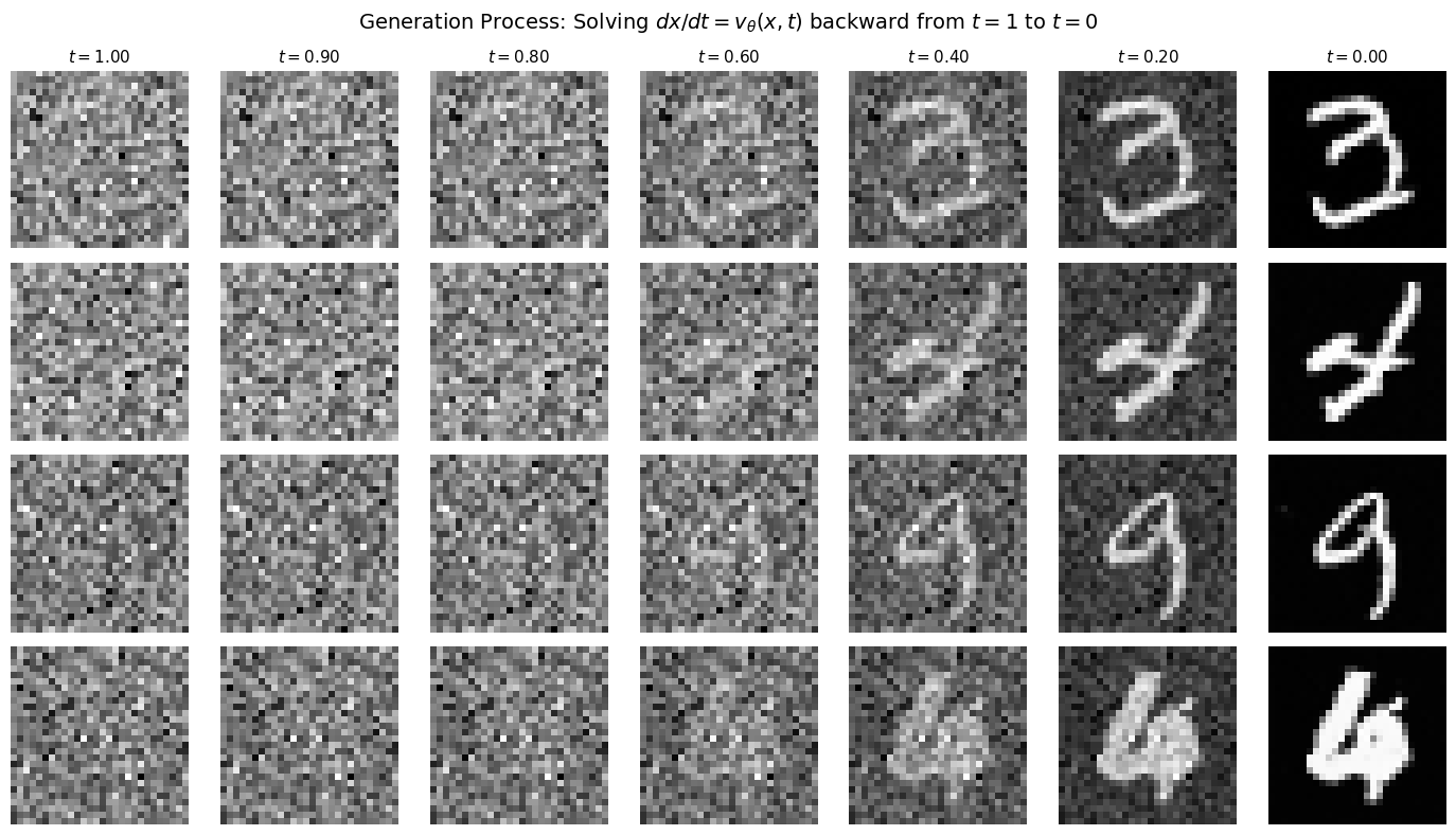


Watch how structure emerges:
• t≈1.0: Random noise (no discernible pattern)
• t≈0.6: Large-scale structure appears (rough digit shape)
• t≈0.3: Details emerge (strokes, curves)
• t=0.0: Final digit

Step 8: Analyzing What the Model Learned¶

Let’s examine how well the model predicts velocities. Remember: the model only sees $x_t$ and $t$ , but must predict $v = x_1 - x_0$ . It can’t know the exact $x_1$ used (since that’s random), so it learns to predict the expected velocity given the noisy input.

# Compare predicted vs true velocity
x_0 = sample_batch[0:1].to(device)
x_1 = torch.randn_like(x_0)
t = torch.tensor([0.5], device=device)

# True velocity
true_v = x_1 - x_0

# Interpolated sample
x_t = (1 - t.view(-1, 1, 1, 1)) * x_0 + t.view(-1, 1, 1, 1) * x_1

# Predicted velocity
model.eval()
with torch.no_grad():
    pred_v = model(x_t, t)

# Visualize
fig, axes = plt.subplots(2, 3, figsize=(14, 8))

# Top row: the samples
axes[0, 0].imshow((x_0[0, 0].cpu() + 1) / 2, cmap='gray')
axes[0, 0].set_title('$x_0$ (data)', fontsize=12)
axes[0, 0].axis('off')

axes[0, 1].imshow((x_t[0, 0].cpu() + 1) / 2, cmap='gray')
axes[0, 1].set_title('$x_t$ at $t=0.5$\n(model input)', fontsize=12)
axes[0, 1].axis('off')

axes[0, 2].imshow((x_1[0, 0].cpu() + 1) / 2, cmap='gray')
axes[0, 2].set_title('$x_1$ (noise)', fontsize=12)
axes[0, 2].axis('off')

# Bottom row: velocities
vmin, vmax = -2, 2

im = axes[1, 0].imshow(true_v[0, 0].cpu(), cmap='RdBu', vmin=vmin, vmax=vmax)
axes[1, 0].set_title('True $v = x_1 - x_0$', fontsize=12)
axes[1, 0].axis('off')

axes[1, 1].imshow(pred_v[0, 0].cpu(), cmap='RdBu', vmin=vmin, vmax=vmax)
axes[1, 1].set_title('Predicted $v_\\theta(x_t, t)$', fontsize=12)
axes[1, 1].axis('off')

error = (pred_v - true_v)[0, 0].cpu()
axes[1, 2].imshow(error, cmap='RdBu', vmin=-1, vmax=1)
axes[1, 2].set_title(f'Error (MSE={torch.mean(error**2):.4f})', fontsize=12)
axes[1, 2].axis('off')

plt.colorbar(im, ax=axes[1, :], orientation='horizontal', fraction=0.05, pad=0.1)
plt.suptitle('Velocity Prediction Analysis', fontsize=14)
plt.show()

print("\nThe model sees only x_t and t, but must predict v = x_1 - x_0.")
print("It can't know the exact x_1 used, so it predicts the expected velocity.")
print("The prediction captures overall structure even if not pixel-perfect.")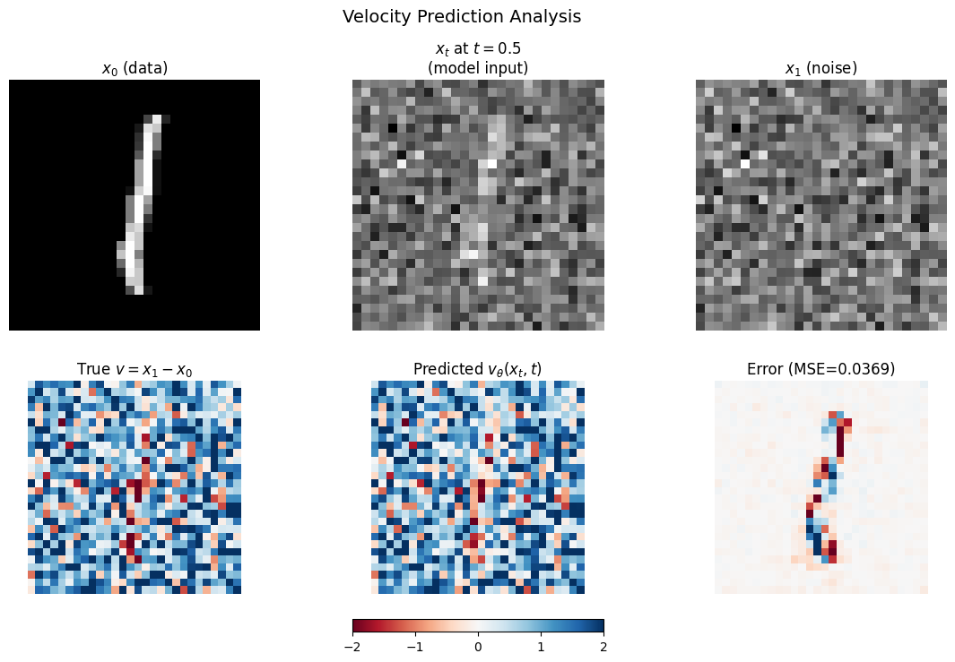


The model sees only x_t and t, but must predict v = x_1 - x_0.
It can't know the exact x_1 used, so it predicts the expected velocity.
The prediction captures overall structure even if not pixel-perfect.

# Save the trained model for use in the next notebook
trainer.save_checkpoint("phase1_model.pt")
print("Model saved to phase1_model.pt")

Model saved to phase1_model.pt

Summary: The Flow Matching Recipe¶

We’ve built a complete generative model using flow matching. Here’s the recipe:

The Framework¶

Step	What Happens
1. Define the path	Linear interpolation $x_t = (1-t)x_0 + tx_1$
2. Compute velocity	Constant $v = x_1 - x_0$
3. Train	Learn $v_\theta(x_t, t) \approx v$ via MSE
4. Sample	Solve ODE backward from $t=1$ to $t=0$

Key Mathematical Insights¶

Concept	Why It Matters
Linear interpolation	Simplest path, constant velocity, optimal transport
Constant velocity	No acceleration = efficient integration
MSE loss	Directly measures velocity prediction quality
Deterministic ODE	Unlike DDPM, no stochastic noise during sampling

Limitations (So Far)¶

Unconditional: We can’t control which digit gets generated
CNN architecture: U-Net works but doesn’t scale as well as transformers
Small scale: More training and larger models would help quality

What’s Next¶

In the following notebooks, we’ll address these limitations:

Notebook 02: Diffusion Transformer (DiT)

Replace the U-Net with a transformer
Patchify images into sequences
Use adaptive layer normalization (adaLN) for conditioning

Notebook 03: Class Conditioning

Control which digit gets generated
Classifier-free guidance for stronger conditioning

Notebook 04: Text Conditioning

CLIP text encoder integration
Cross-attention for text-to-image

Notebook 05: Latent Diffusion

Work in compressed latent space
VAE encoder/decoder
The Stable Diffusion approach