Latent Diffusion: Compressing the Problem - An Introduction to Transformers

We’ve built a complete diffusion pipeline—flow matching, transformers, class conditioning, text conditioning. There’s just one problem: it doesn’t scale.

Try running our DiT on a 512×512 image. Go ahead, I’ll wait. Actually, don’t—your GPU will run out of memory before you can say “attention complexity.”

This is where latent diffusion comes in. The key insight (from Rombach et al., 2022) is almost embarrassingly simple: what if we did diffusion in a smaller space?

The Scaling Wall¶

Let’s look at the numbers:

Resolution	Pixels	Patches (4×4)	Attention Pairs
32×32	3,072	64	4,096
64×64	12,288	256	65,536
256×256	196,608	4,096	16,777,216
512×512	786,432	16,384	268,435,456

Self-attention is $O(N^2)$ in sequence length. Going from 32×32 to 512×512 increases attention cost by 65,536×. That’s not a typo.

Even with tricks like efficient attention, this is brutal. We need a fundamentally different approach.

The Latent Diffusion Solution¶

The solution has two parts:

Compress images to a small latent space using a pretrained autoencoder
Diffuse in that latent space instead of pixel space

Pixel-Space Diffusion:
  noise (512×512×3) ──[50 DiT steps]──> image (512×512×3)
  
Latent-Space Diffusion:
  noise (64×64×4) ──[50 DiT steps]──> latent (64×64×4) ──[VAE decode]──> image (512×512×3)

With 8× spatial compression:

512×512×3 → 64×64×4 latents
786,432 → 16,384 dimensions (48× smaller)
16,384 tokens → 1,024 tokens (16× fewer)
Attention cost drops by 256×

The expensive ODE integration happens in the compressed space. The autoencoder (run just once at the end) handles the decompression.

What We’ll Build¶

Variational Autoencoder (VAE): The compression engine
The Reparameterization Trick: How to backpropagate through randomness
Latent Flow Matching: Our familiar pipeline, now in compressed space
The Complete System: Encode → Denoise → Decode

By the end, you’ll understand exactly how Stable Diffusion works.

import torch
import torch.nn as nn
import torch.nn.functional as F
import torchvision
import torchvision.transforms as transforms
from torch.utils.data import DataLoader
import matplotlib.pyplot as plt
import numpy as np

%load_ext autoreload
%autoreload 2

from from_noise_to_images import get_device
device = get_device()
print(f"Using device: {device}")

Using device: cuda

Part 1: The Variational Autoencoder¶

A VAE learns to compress images into a smaller latent space and decompress them back. But it’s not just any autoencoder—it’s probabilistic.

Why Not a Regular Autoencoder?¶

A regular autoencoder learns:

x \xrightarrow{\text{encode}} z \xrightarrow{\text{decode}} \hat{x}

(1)

Train with reconstruction loss $\|x - \hat{x}\|^2$ , done. But there’s a problem.

The latent space of a regular autoencoder can have holes—regions where no training image maps to. If you sample from such a region and decode, you get garbage. The encoder just memorizes where to put each training image; it doesn’t organize the space nicely.

For diffusion, this is fatal. We’re going to sample noise $z \sim \mathcal{N}(0, I)$ and decode it. We need every region of latent space to decode to something reasonable.

The VAE Solution: Probabilistic Encoding¶

A VAE encodes to a distribution, not a point:

x \xrightarrow{\text{encode}} (\mu, \sigma^2) \xrightarrow{\text{sample}} z \xrightarrow{\text{decode}} \hat{x}

(2)

The encoder outputs parameters of a Gaussian: mean $\mu$ and variance $\sigma^2$ . We then sample from that Gaussian to get $z$ .

The ELBO: Reconstruction + Regularization¶

The VAE training objective comes from variational inference. We want to maximize the likelihood of our data, but that’s intractable. Instead, we maximize a lower bound (ELBO):

\log p(x) \geq \underbrace{\mathbb{E}_{q(z|x)}[\log p(x|z)]}_{\text{reconstruction}} - \underbrace{D_{KL}(q(z|x) \| p(z))}_{\text{regularization}}

(3)

In practice, we minimize:

\mathcal{L}_{\text{VAE}} = \underbrace{\|x - \hat{x}\|^2}_{\text{reconstruction}} + \beta \cdot \underbrace{D_{KL}(q(z|x) \| \mathcal{N}(0, I))}_{\text{KL penalty}}

(4)

Reconstruction loss: Make the decoded output match the input.

KL divergence: Force the encoder distribution $q(z|x) = \mathcal{N}(\mu, \sigma^2)$ to be close to the prior $p(z) = \mathcal{N}(0, I)$ .

Why the KL Term Helps¶

The KL penalty:

Fills holes: Pushes all encoder distributions toward $\mathcal{N}(0, I)$ , ensuring coverage
Smooths the space: Nearby points in latent space decode to similar images
Enables sampling: We can sample $z \sim \mathcal{N}(0, I)$ and decode to valid images

KL Divergence for Gaussians¶

For $q(z|x) = \mathcal{N}(\mu, \sigma^2)$ and $p(z) = \mathcal{N}(0, I)$ :

D_{KL} = -\frac{1}{2} \sum_{i=1}^{d} \left(1 + \log\sigma_i^2 - \mu_i^2 - \sigma_i^2\right)

(5)

Let’s verify this makes sense:

If $\mu = 0$ and $\sigma = 1$ : $D_{KL} = 0$ (perfect match)
If $\mu \neq 0$ : $D_{KL}$ increases (penalizes shifted mean)
If $\sigma \neq 1$ : $D_{KL}$ increases (penalizes wrong variance)

# Let's verify the KL divergence formula
def kl_divergence(mu, logvar):
    """KL divergence from N(mu, sigma^2) to N(0, 1).
    
    Using log-variance for numerical stability.
    sigma^2 = exp(logvar)
    """
    return -0.5 * torch.sum(1 + logvar - mu.pow(2) - logvar.exp())

# Test different scenarios
scenarios = [
    ("μ=0, σ=1 (perfect match to prior)", 0.0, 0.0),
    ("μ=1, σ=1 (shifted mean)", 1.0, 0.0),
    ("μ=0, σ=0.5 (too narrow)", 0.0, np.log(0.25)),
    ("μ=0, σ=2.0 (too wide)", 0.0, np.log(4.0)),
    ("μ=2, σ=0.5 (shifted + narrow)", 2.0, np.log(0.25)),
]

print("KL Divergence from N(μ, σ²) to N(0, 1):")
print("=" * 55)
for name, mu_val, logvar_val in scenarios:
    mu = torch.tensor([mu_val])
    logvar = torch.tensor([logvar_val])
    kl = kl_divergence(mu, logvar).item()
    print(f"{name:40s}  KL = {kl:.4f}")

print()
print("The KL term pushes the encoder toward μ=0, σ=1.")
print("Any deviation increases the loss.")

KL Divergence from N(μ, σ²) to N(0, 1):
=======================================================
μ=0, σ=1 (perfect match to prior)         KL = -0.0000
μ=1, σ=1 (shifted mean)                   KL = 0.5000
μ=0, σ=0.5 (too narrow)                   KL = 0.3181
μ=0, σ=2.0 (too wide)                     KL = 0.8069
μ=2, σ=0.5 (shifted + narrow)             KL = 2.3181

The KL term pushes the encoder toward μ=0, σ=1.
Any deviation increases the loss.

The Reparameterization Trick¶

Here’s a problem: the encoder outputs $(\mu, \sigma^2)$ , and we sample $z \sim \mathcal{N}(\mu, \sigma^2)$ . But sampling is a random operation—how do we backpropagate through it?

The trick: rewrite the sampling as a deterministic function plus external noise:

z = \mu + \sigma \cdot \epsilon, \quad \epsilon \sim \mathcal{N}(0, I)

(6)

Now $z$ is a deterministic function of $\mu$ , $\sigma$ , and $\epsilon$ . The randomness ( $\epsilon$ ) is sampled independently and treated as a constant during backprop.

Gradients flow through:

\frac{\partial z}{\partial \mu} = 1, \quad \frac{\partial z}{\partial \sigma} = \epsilon

(7)

In code:

def reparameterize(mu, logvar):
    std = torch.exp(0.5 * logvar)  # σ = exp(log(σ²)/2)
    eps = torch.randn_like(std)     # ε ~ N(0, I)
    return mu + std * eps           # z = μ + σε

We use logvar (log-variance) instead of variance directly for numerical stability—it can be any real number, while variance must be positive.

# Demonstrate the reparameterization trick
def reparameterize(mu, logvar):
    """Sample z = μ + σε where ε ~ N(0, I)."""
    std = torch.exp(0.5 * logvar)  # σ = sqrt(exp(logvar))
    eps = torch.randn_like(std)
    return mu + std * eps

# Test
mu = torch.tensor([2.0], requires_grad=True)
logvar = torch.tensor([0.0], requires_grad=True)  # σ = 1

torch.manual_seed(42)
z = reparameterize(mu, logvar)

print(f"μ = {mu.item():.2f}")
print(f"σ = {torch.exp(0.5 * logvar).item():.2f}")
print(f"z = {z.item():.4f}")
print()

# Check gradients exist
loss = z.sum()
loss.backward()

print(f"∂z/∂μ = {mu.grad.item():.2f} (should be 1)")
print(f"∂z/∂logvar = {logvar.grad.item():.4f} (depends on ε)")
print()
print("Gradients flow through! The trick works.")

μ = 2.00
σ = 1.00
z = 2.3367

∂z/∂μ = 1.00 (should be 1)
∂z/∂logvar = 0.1683 (depends on ε)

Gradients flow through! The trick works.

Part 2: Building and Training the VAE¶

Let’s train a VAE on CIFAR-10 (32×32 RGB images). Our architecture:

Encoder (32×32 → 8×8, 4× spatial compression):

Conv: 3 → 64 channels
Downsample: 64 → 64, stride 2 (32→16)
Downsample: 64 → 128, stride 2 (16→8)
Conv: 128 → 8 (4 for μ, 4 for log σ²)

Decoder (8×8 → 32×32):

Conv: 4 → 128 channels
Upsample: 128 → 64, ×2 (8→16)
Upsample: 64 → 64, ×2 (16→32)
Conv: 64 → 3

Compression:

Input: 32×32×3 = 3,072 values
Latent: 8×8×4 = 256 values
12× compression

# Load CIFAR-10
transform = transforms.Compose([
    transforms.ToTensor(),
    transforms.Normalize((0.5, 0.5, 0.5), (0.5, 0.5, 0.5))  # [-1, 1]
])

train_dataset = torchvision.datasets.CIFAR10(
    root="./data",
    train=True,
    download=True,
    transform=transform
)

train_loader = DataLoader(
    train_dataset,
    batch_size=128,
    shuffle=True,
    num_workers=0,
    drop_last=True
)

print(f"Dataset: {len(train_dataset):,} images")
print(f"Shape: {train_dataset[0][0].shape} (C, H, W)")
print(f"Range: [{train_dataset[0][0].min():.1f}, {train_dataset[0][0].max():.1f}]")

Dataset: 50,000 images
Shape: torch.Size([3, 32, 32]) (C, H, W)
Range: [-1.0, 1.0]

def show_images(images, nrow=8, title=""):
    """Display a grid of images."""
    images = (images + 1) / 2  # [-1, 1] → [0, 1]
    images = images.clamp(0, 1)
    
    grid = torchvision.utils.make_grid(images, nrow=nrow, padding=2)
    plt.figure(figsize=(12, 12 * grid.shape[1] / grid.shape[2]))
    plt.imshow(grid.permute(1, 2, 0).cpu().numpy())
    plt.axis('off')
    if title:
        plt.title(title, fontsize=14)
    plt.show()

sample_batch, sample_labels = next(iter(train_loader))
show_images(sample_batch[:32], title="CIFAR-10 Training Images")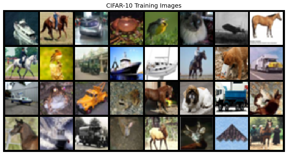

from from_noise_to_images.vae import SmallVAE

vae = SmallVAE(
    in_channels=3,
    latent_channels=4,
    hidden_channels=64,
).to(device)

num_params = sum(p.numel() for p in vae.parameters() if p.requires_grad)
print(f"VAE parameters: {num_params:,}")
print()

# Test forward pass
test_img = torch.randn(4, 3, 32, 32, device=device)
with torch.no_grad():
    recon, mean, logvar = vae(test_img)
    latent = vae.encode(test_img)

print("Shape analysis:")
print(f"  Input:  {test_img.shape}  ({test_img[0].numel():,} values)")
print(f"  μ, σ²:  {mean.shape}  ({mean[0].numel():,} values each)")
print(f"  Latent: {latent.shape}  ({latent[0].numel():,} values)")
print(f"  Output: {recon.shape}")
print()
print(f"Compression: {test_img[0].numel()} → {latent[0].numel()} = {test_img[0].numel() / latent[0].numel():.0f}×")

VAE parameters: 942,539

Shape analysis:
  Input:  torch.Size([4, 3, 32, 32])  (3,072 values)
  μ, σ²:  torch.Size([4, 4, 8, 8])  (256 values each)
  Latent: torch.Size([4, 4, 8, 8])  (256 values)
  Output: torch.Size([4, 3, 32, 32])

Compression: 3072 → 256 = 12×

Choosing β: Reconstruction vs. Regularization¶

The loss is $\mathcal{L} = \mathcal{L}_{\text{recon}} + \beta \cdot D_{KL}$ .

β Value	Behavior	Use Case
β = 1	Standard VAE	General generative modeling
β > 1	Disentangled latents	β-VAE for interpretable features
β ≪ 1	Prioritize reconstruction	Latent diffusion

For latent diffusion, we use β ≈ 10⁻⁵. Why so small?

Reconstruction quality matters most: The decoder needs to produce sharp images from latents
The diffusion model handles generation: We don’t need to sample directly from N(0, I)
Latent statistics: We’ll compute a scale factor to normalize the latent space anyway

With tiny β, the VAE is almost a regular autoencoder with a slight push toward organized latents.

from from_noise_to_images.train import VAETrainer

vae_trainer = VAETrainer(
    model=vae,
    dataloader=train_loader,
    lr=1e-4,
    weight_decay=0.01,
    kl_weight=0.00001,  # Very small β for latent diffusion
    device=device,
)

VAE_EPOCHS = 30
print(f"Training VAE for {VAE_EPOCHS} epochs")
print(f"β (KL weight) = {vae_trainer.kl_weight}")
print()

vae_losses = vae_trainer.train(num_epochs=VAE_EPOCHS)

Training VAE for 30 epochs
β (KL weight) = 1e-05

Training VAE on cuda
Model parameters: 942,539
KL weight (β): 1e-05

Epoch 1: loss=0.0590, recon=0.0547, kl=431.1141

Epoch 2: loss=0.0293, recon=0.0242, kl=502.6520

Epoch 3: loss=0.0253, recon=0.0202, kl=503.5774

Epoch 4: loss=0.0222, recon=0.0171, kl=508.3687

Epoch 5: loss=0.0207, recon=0.0156, kl=505.6616

Epoch 6: loss=0.0198, recon=0.0148, kl=501.7215

Epoch 7: loss=0.0192, recon=0.0142, kl=498.4863

Epoch 8: loss=0.0187, recon=0.0137, kl=495.4255

Epoch 9: loss=0.0183, recon=0.0134, kl=492.8486

Epoch 10: loss=0.0180, recon=0.0131, kl=490.3126

Epoch 11: loss=0.0177, recon=0.0128, kl=487.9923

Epoch 12: loss=0.0174, recon=0.0125, kl=485.8511

Epoch 13: loss=0.0172, recon=0.0124, kl=483.7837

Epoch 14: loss=0.0170, recon=0.0122, kl=481.8108

Epoch 15: loss=0.0169, recon=0.0121, kl=479.9993

Epoch 16: loss=0.0167, recon=0.0119, kl=478.1108

Epoch 17: loss=0.0165, recon=0.0118, kl=476.5316

Epoch 18: loss=0.0164, recon=0.0117, kl=475.1542

Epoch 19: loss=0.0163, recon=0.0116, kl=473.9001

Epoch 20: loss=0.0162, recon=0.0115, kl=472.7261

Epoch 21: loss=0.0161, recon=0.0114, kl=471.5731

Epoch 22: loss=0.0160, recon=0.0113, kl=470.4031

Epoch 23: loss=0.0159, recon=0.0112, kl=469.6428

Epoch 24: loss=0.0158, recon=0.0112, kl=468.9225

Epoch 25: loss=0.0158, recon=0.0111, kl=468.1379

Epoch 26: loss=0.0157, recon=0.0110, kl=467.5905

Epoch 27: loss=0.0156, recon=0.0110, kl=466.9360

Epoch 28: loss=0.0156, recon=0.0109, kl=466.3908

Epoch 29: loss=0.0155, recon=0.0108, kl=465.9495

Epoch 30: loss=0.0155, recon=0.0108, kl=465.5777

Computing latent scale factor...

Scale factor: 0.9692

fig, axes = plt.subplots(1, 2, figsize=(12, 4))

axes[0].plot(vae_trainer.losses, label='Total')
axes[0].plot(vae_trainer.recon_losses, label='Reconstruction')
axes[0].set_xlabel('Epoch')
axes[0].set_ylabel('Loss')
axes[0].set_title('VAE Training Loss')
axes[0].legend()
axes[0].grid(True, alpha=0.3)

axes[1].plot(vae_trainer.kl_losses)
axes[1].set_xlabel('Epoch')
axes[1].set_ylabel('KL Divergence')
axes[1].set_title('KL Divergence (Raw, Before β Scaling)')
axes[1].grid(True, alpha=0.3)

plt.tight_layout()
plt.show()

print(f"Final reconstruction loss: {vae_trainer.recon_losses[-1]:.4f}")
print(f"Final KL (raw): {vae_trainer.kl_losses[-1]:.1f}")
print(f"Final KL (weighted): {vae_trainer.kl_losses[-1] * vae_trainer.kl_weight:.6f}")

Final reconstruction loss: 0.0108
Final KL (raw): 465.6
Final KL (weighted): 0.004656

# Visualize reconstructions
vae.eval()

test_batch = sample_batch[:16].to(device)

with torch.no_grad():
    recon, _, _ = vae(test_batch)

fig, axes = plt.subplots(2, 1, figsize=(14, 7))

original_grid = torchvision.utils.make_grid((test_batch + 1) / 2, nrow=16, padding=2)
axes[0].imshow(original_grid.permute(1, 2, 0).cpu().numpy())
axes[0].set_title('Original (32×32×3 = 3,072 values)', fontsize=12)
axes[0].axis('off')

recon_grid = torchvision.utils.make_grid((recon + 1) / 2, nrow=16, padding=2)
axes[1].imshow(recon_grid.permute(1, 2, 0).cpu().clamp(0, 1).numpy())
axes[1].set_title('Reconstructed via 8×8×4 = 256 latent values (12× compression)', fontsize=12)
axes[1].axis('off')

plt.tight_layout()
plt.show()

mse = F.mse_loss(recon, test_batch).item()
print(f"Reconstruction MSE: {mse:.4f}")

Reconstruction MSE: 0.0113

Part 3: Exploring the Latent Space¶

Before we do diffusion, let’s understand what the latent space looks like.

Scale Factor¶

Remember, we used a tiny β, so the latent space isn’t perfectly $\mathcal{N}(0, I)$ . We need to normalize it.

After training, we compute the empirical standard deviation:

\sigma_{\text{data}} = \text{std}(\{\text{encode}(x) : x \in \text{training set}\})

(8)

Then normalize latents:

z_{\text{normalized}} = z / \sigma_{\text{data}}

(9)

This ensures the latent space roughly matches the noise distribution $\mathcal{N}(0, I)$ we’ll use for flow matching.

# Analyze latent space statistics
vae.eval()

all_means = []
all_stds = []

with torch.no_grad():
    for i, (images, _) in enumerate(train_loader):
        if i >= 50:
            break
        images = images.to(device)
        z = vae.encode(images, sample=False)  # Use mean (no sampling noise)
        all_means.append(z.mean().item())
        all_stds.append(z.std().item())

avg_mean = np.mean(all_means)
avg_std = np.mean(all_stds)

print("Latent Space Statistics (before normalization):")
print(f"  Mean: {avg_mean:.4f} (target: 0)")
print(f"  Std:  {avg_std:.4f} (will normalize to ~1)")
print()
print(f"VAE computed scale factor: {vae.scale_factor.item():.4f}")
print("(Latents are divided by this during encoding)")

Latent Space Statistics (before normalization):
  Mean: -0.0144 (target: 0)
  Std:  0.9991 (will normalize to ~1)

VAE computed scale factor: 0.9692
(Latents are divided by this during encoding)

# Visualize what the latent channels capture
test_img = sample_batch[0:1].to(device)

with torch.no_grad():
    z = vae.encode(test_img, sample=False)

fig, axes = plt.subplots(1, 5, figsize=(15, 3))

# Original
axes[0].imshow((test_img[0].cpu().permute(1, 2, 0) + 1) / 2)
axes[0].set_title('Original\n(32×32×3)')
axes[0].axis('off')

# Each latent channel
for i in range(4):
    latent_ch = z[0, i].cpu().numpy()
    axes[i+1].imshow(latent_ch, cmap='RdBu', vmin=-2, vmax=2)
    axes[i+1].set_title(f'Latent Ch {i}\n(8×8)')
    axes[i+1].axis('off')

plt.suptitle('The VAE Compresses 32×32×3 → 8×8×4 (12× fewer values)', fontsize=12)
plt.tight_layout()
plt.show()

print(f"Latent shape: {z.shape}")
print(f"Latent range: [{z.min():.2f}, {z.max():.2f}]")
print()
print("Each 8×8 channel captures different aspects of the image.")
print("The decoder learns to reconstruct the full image from these 256 numbers.")

Latent shape: torch.Size([1, 4, 8, 8])
Latent range: [-2.47, 3.14]

Each 8×8 channel captures different aspects of the image.
The decoder learns to reconstruct the full image from these 256 numbers.

Part 4: Flow Matching in Latent Space¶

Now for the main event. We’ll train a DiT to do flow matching, but in the latent space instead of pixel space.

The Key Substitution¶

Everything works exactly as before, just with latents instead of pixels:

Pixel Space	Latent Space
$x_0$ = image	$z_0$ = encode(image)
$x_1 \sim \mathcal{N}(0, I)$	$z_1 \sim \mathcal{N}(0, I)$
$x_t = (1-t)x_0 + tx_1$	$z_t = (1-t)z_0 + tz_1$
$v = x_1 - x_0$	$v = z_1 - z_0$
Generate $x$ directly	Generate $z$ , then decode

DiT for Latent Space¶

The DiT now operates on the smaller latent shape:

in_channels=4 (latent channels, not RGB)
img_size=8 (latent spatial size, not image size)
patch_size=2 → 16 tokens (not 64)

The Computational Win¶

Metric	Pixel Space	Latent Space	Reduction
Input size	32×32×3 = 3,072	8×8×4 = 256	12×
Tokens (patch=2)	16×16 = 256	4×4 = 16	16×
Attention pairs	65,536	256	256×

from from_noise_to_images.dit import DiT

# DiT for latent space
latent_dit = DiT(
    img_size=8,           # Latent spatial size
    patch_size=2,         # 2×2 patches → 4×4 = 16 tokens
    in_channels=4,        # Latent channels
    embed_dim=256,
    depth=6,
    num_heads=8,
    mlp_ratio=4.0,
).to(device)

latent_dit_params = sum(p.numel() for p in latent_dit.parameters())

# For comparison: pixel-space DiT
pixel_dit = DiT(
    img_size=32,
    patch_size=4,
    in_channels=3,
    embed_dim=256,
    depth=6,
    num_heads=8,
)
pixel_dit_params = sum(p.numel() for p in pixel_dit.parameters())

print("Comparison:")
print(f"  Pixel-space DiT: {pixel_dit_params:,} params, {8*8}=64 tokens")
print(f"  Latent-space DiT: {latent_dit_params:,} params, {4*4}=16 tokens")
print()
print(f"Token reduction: {64/16:.0f}×")
print(f"Attention cost reduction: {(64*64)/(16*16):.0f}×")
print()
print("Same parameter count, but 16× fewer attention computations per step!")

Comparison:
  Pixel-space DiT: 12,368,176 params, 64=64 tokens
  Latent-space DiT: 12,351,760 params, 16=16 tokens

Token reduction: 4×
Attention cost reduction: 16×

Same parameter count, but 16× fewer attention computations per step!

from from_noise_to_images.train import LatentDiffusionTrainer

latent_trainer = LatentDiffusionTrainer(
    model=latent_dit,
    vae=vae,  # VAE is frozen, used only for encoding
    dataloader=train_loader,
    lr=1e-4,
    weight_decay=0.01,
    device=device,
)

LATENT_EPOCHS = 30
print(f"Training Latent DiT for {LATENT_EPOCHS} epochs")
print("VAE is frozen—only DiT parameters are trained.")
print()

latent_losses = latent_trainer.train(num_epochs=LATENT_EPOCHS)

Training Latent DiT for 30 epochs
VAE is frozen—only DiT parameters are trained.

Training Latent Diffusion on cuda
DiT parameters: 12,351,760
VAE parameters: 0 (frozen)

Epoch 1: avg_loss = 1.6264

Epoch 2: avg_loss = 1.4547

Epoch 3: avg_loss = 1.4348

Epoch 4: avg_loss = 1.4271

Epoch 5: avg_loss = 1.4166

Epoch 6: avg_loss = 1.4125

Epoch 7: avg_loss = 1.4074

Epoch 8: avg_loss = 1.4011

Epoch 9: avg_loss = 1.3978

Epoch 10: avg_loss = 1.3939

Epoch 11: avg_loss = 1.3927

Epoch 12: avg_loss = 1.3877

Epoch 13: avg_loss = 1.3872

Epoch 14: avg_loss = 1.3826

Epoch 15: avg_loss = 1.3805

Epoch 16: avg_loss = 1.3762

Epoch 17: avg_loss = 1.3741

Epoch 18: avg_loss = 1.3714

Epoch 19: avg_loss = 1.3703

Epoch 20: avg_loss = 1.3664

Epoch 21: avg_loss = 1.3655

Epoch 22: avg_loss = 1.3648

Epoch 23: avg_loss = 1.3630

Epoch 24: avg_loss = 1.3621

Epoch 25: avg_loss = 1.3596

Epoch 26: avg_loss = 1.3585

Epoch 27: avg_loss = 1.3583

Epoch 28: avg_loss = 1.3554

Epoch 29: avg_loss = 1.3538

Epoch 30: avg_loss = 1.3546

plt.figure(figsize=(10, 4))
plt.plot(latent_losses)
plt.xlabel('Epoch')
plt.ylabel('MSE Loss (velocity prediction)')
plt.title('Latent Diffusion Training')
plt.grid(True, alpha=0.3)
plt.show()

print(f"Final loss: {latent_losses[-1]:.4f}")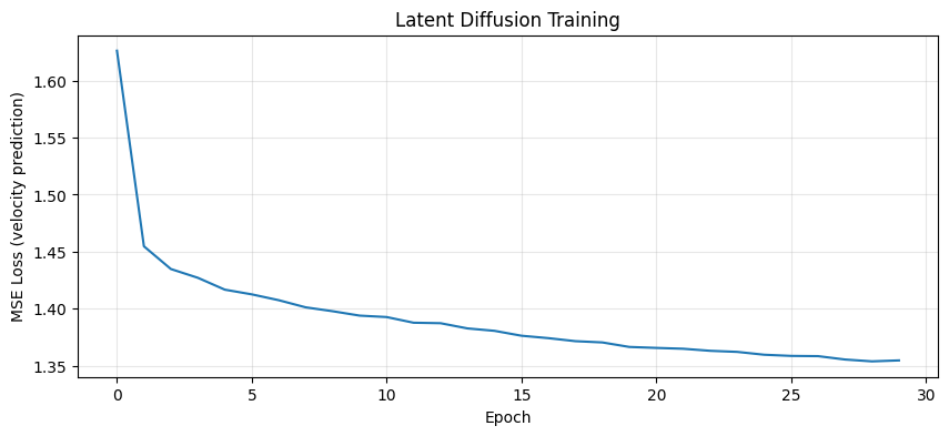

Final loss: 1.3546

Part 5: Sampling from Latent Space¶

Generation in latent diffusion:

Sample noise in latent space: $z_1 \sim \mathcal{N}(0, I)$ , shape (4, 8, 8)
Integrate ODE: $z_1 \to z_0$ using learned velocity
Decode to pixels: $x = \text{decode}(z_0)$ , shape (3, 32, 32)

All the expensive ODE steps (50 forward passes) happen in the small 256-dimensional latent space. The VAE decode (one forward pass) happens only at the end.

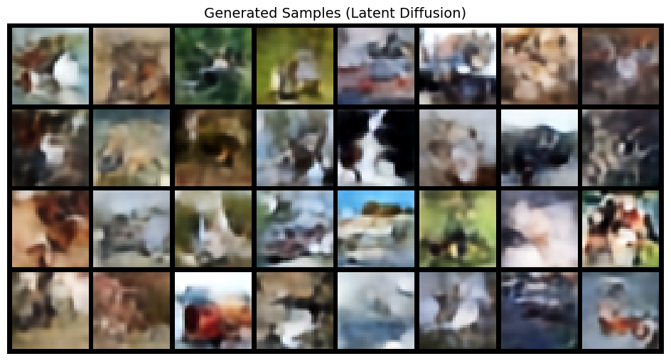
from from_noise_to_images.sampling import sample_latent

latent_dit.eval()
vae.eval()

print("Generation pipeline:")
print("  1. Sample z₁ ~ N(0, I) in latent space (4×8×8 = 256 dim)")
print("  2. ODE: z₁ → z₀ via 50 Euler steps")
print("  3. Decode: z₀ → image via VAE (3×32×32 = 3,072 dim)")
print()

with torch.no_grad():
    generated = sample_latent(
        model=latent_dit,
        vae=vae,
        num_samples=32,
        latent_shape=(4, 8, 8),
        num_steps=50,
        device=device,
    )

show_images(generated, nrow=8, title="Generated Samples (Latent Diffusion)")

Generation pipeline:
  1. Sample z₁ ~ N(0, I) in latent space (4×8×8 = 256 dim)
  2. ODE: z₁ → z₀ via 50 Euler steps
  3. Decode: z₀ → image via VAE (3×32×32 = 3,072 dim)

# Visualize the generation process
with torch.no_grad():
    generated, trajectory = sample_latent(
        model=latent_dit,
        vae=vae,
        num_samples=4,
        latent_shape=(4, 8, 8),
        num_steps=50,
        device=device,
        return_trajectory=True,
    )

# Show evolution
steps_to_show = [0, 10, 20, 30, 40, 50]
fig, axes = plt.subplots(2, len(steps_to_show), figsize=(15, 6))

for col, step_idx in enumerate(steps_to_show):
    t_val = 1.0 - step_idx / 50
    
    # Latent (first channel)
    latent = trajectory[step_idx][0, 0].cpu().numpy()
    axes[0, col].imshow(latent, cmap='RdBu', vmin=-3, vmax=3)
    axes[0, col].set_title(f't={t_val:.2f}')
    axes[0, col].axis('off')
    
    # Decoded image
    with torch.no_grad():
        decoded = vae.decode(trajectory[step_idx][:1])
    img = (decoded[0].cpu().permute(1, 2, 0) + 1) / 2
    axes[1, col].imshow(img.clamp(0, 1).numpy())
    axes[1, col].axis('off')

axes[0, 0].set_ylabel('Latent\n(8×8)', fontsize=10)
axes[1, 0].set_ylabel('Decoded\n(32×32)', fontsize=10)

plt.suptitle('Latent Diffusion: ODE Integration in Latent Space', fontsize=12)
plt.tight_layout()
plt.show()

print("At t=1: Pure noise in latent space → noisy decode")
print("At t→0: Structure emerges in latent → coherent image")
print()
print("The key insight: all 50 ODE steps happen in 256-dim space,")
print("not 3,072-dim pixel space. That's the efficiency win.")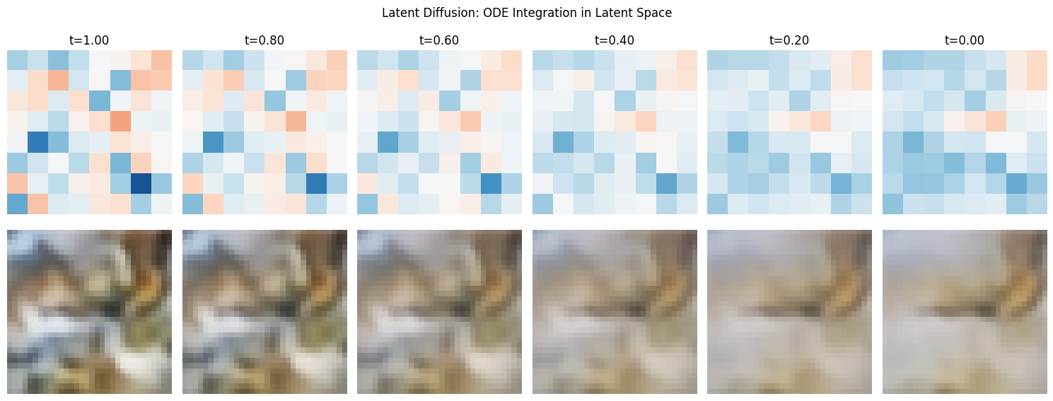

At t=1: Pure noise in latent space → noisy decode
At t→0: Structure emerges in latent → coherent image

The key insight: all 50 ODE steps happen in 256-dim space,
not 3,072-dim pixel space. That's the efficiency win.

Part 6: Class-Conditional Latent Diffusion¶

We can add conditioning to latent diffusion just like we did in the pixel-space version. The architecture is identical—we’re just operating on latent shapes.

from from_noise_to_images.dit import ConditionalDiT

cond_latent_dit = ConditionalDiT(
    num_classes=10,       # CIFAR-10
    img_size=8,           # Latent spatial size
    patch_size=2,
    in_channels=4,        # Latent channels
    embed_dim=256,
    depth=6,
    num_heads=8,
    mlp_ratio=4.0,
).to(device)

print(f"Conditional Latent DiT: {sum(p.numel() for p in cond_latent_dit.parameters()):,} params")

Conditional Latent DiT: 12,363,024 params

from from_noise_to_images.train import LatentConditionalTrainer

cond_latent_trainer = LatentConditionalTrainer(
    model=cond_latent_dit,
    vae=vae,
    dataloader=train_loader,
    lr=1e-4,
    weight_decay=0.01,
    label_drop_prob=0.1,  # 10% dropout for CFG
    num_classes=10,
    device=device,
)

COND_EPOCHS = 30
print(f"Training Conditional Latent DiT for {COND_EPOCHS} epochs")
print(f"Label dropout: 10% (for Classifier-Free Guidance)")
print()

cond_losses = cond_latent_trainer.train(num_epochs=COND_EPOCHS)

Training Conditional Latent DiT for 30 epochs
Label dropout: 10% (for Classifier-Free Guidance)

Training Latent Conditional Diffusion on cuda
DiT parameters: 12,363,024
CFG label dropout: 10%

Epoch 1: avg_loss = 1.6288

Epoch 2: avg_loss = 1.4465

Epoch 3: avg_loss = 1.4258

Epoch 4: avg_loss = 1.4159

Epoch 5: avg_loss = 1.4078

Epoch 6: avg_loss = 1.4021

Epoch 7: avg_loss = 1.3988

Epoch 8: avg_loss = 1.3929

Epoch 9: avg_loss = 1.3873

Epoch 10: avg_loss = 1.3847

Epoch 11: avg_loss = 1.3814

Epoch 12: avg_loss = 1.3767

Epoch 13: avg_loss = 1.3758

Epoch 14: avg_loss = 1.3735

Epoch 15: avg_loss = 1.3701

Epoch 16: avg_loss = 1.3661

Epoch 17: avg_loss = 1.3651

Epoch 18: avg_loss = 1.3627

Epoch 19: avg_loss = 1.3609

Epoch 20: avg_loss = 1.3564

Epoch 21: avg_loss = 1.3553

Epoch 22: avg_loss = 1.3532

Epoch 23: avg_loss = 1.3527

Epoch 24: avg_loss = 1.3505

Epoch 25: avg_loss = 1.3491

Epoch 26: avg_loss = 1.3473

Epoch 27: avg_loss = 1.3440

Epoch 28: avg_loss = 1.3442

Epoch 29: avg_loss = 1.3432

Epoch 30: avg_loss = 1.3409

from from_noise_to_images.sampling import sample_latent_conditional

CIFAR10_CLASSES = [
    'airplane', 'automobile', 'bird', 'cat', 'deer',
    'dog', 'frog', 'horse', 'ship', 'truck'
]

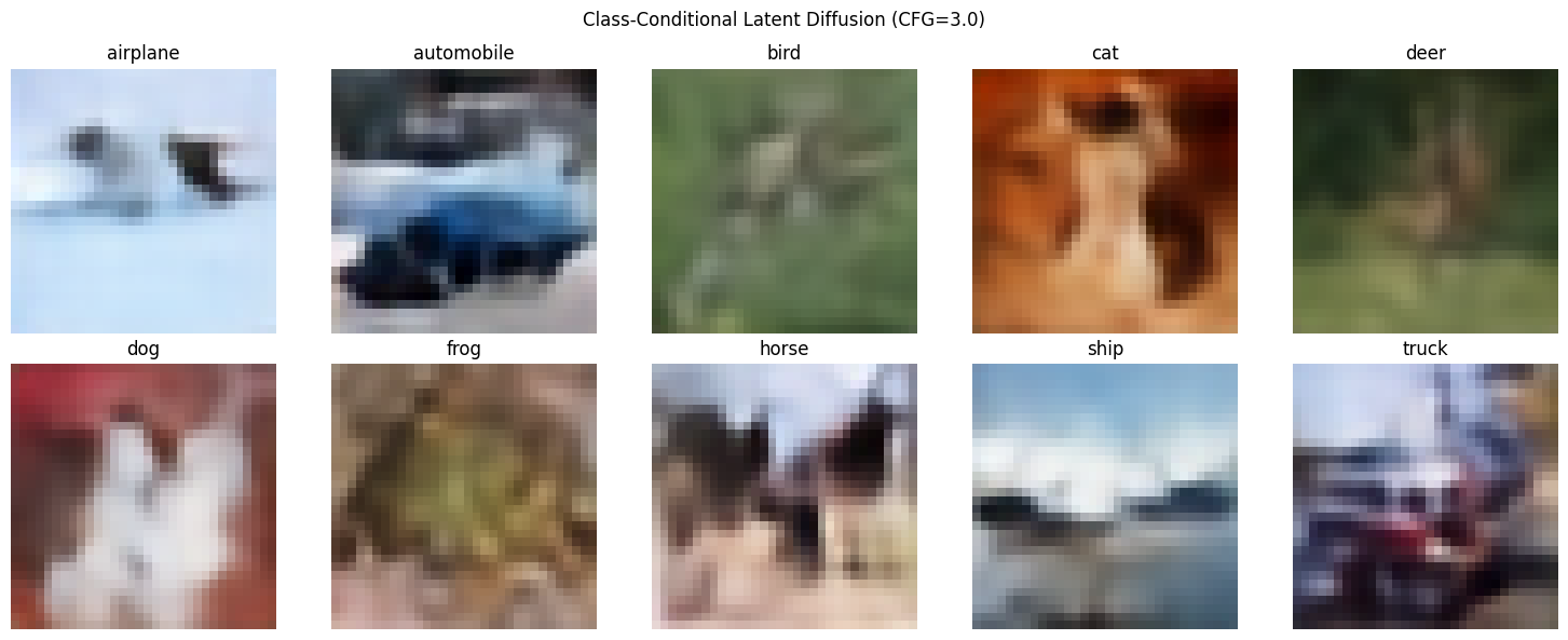
cond_latent_dit.eval()

print("Generating one sample per class with CFG=3.0...")
print()

with torch.no_grad():
    class_samples = sample_latent_conditional(
        model=cond_latent_dit,
        vae=vae,
        class_labels=list(range(10)),
        latent_shape=(4, 8, 8),
        num_steps=50,
        cfg_scale=3.0,
        device=device,
        num_classes=10,
    )

fig, axes = plt.subplots(2, 5, figsize=(15, 6))

for i, (ax, class_name) in enumerate(zip(axes.flat, CIFAR10_CLASSES)):
    img = (class_samples[i].cpu().permute(1, 2, 0) + 1) / 2
    ax.imshow(img.clamp(0, 1).numpy())
    ax.set_title(class_name)
    ax.axis('off')

plt.suptitle('Class-Conditional Latent Diffusion (CFG=3.0)', fontsize=12)
plt.tight_layout()
plt.show()

Generating one sample per class with CFG=3.0...

# Compare CFG scales
cfg_scales = [1.0, 2.0, 3.0, 5.0]
target_class = 3  # cat

fig, axes = plt.subplots(1, len(cfg_scales), figsize=(16, 4))

for ax, scale in zip(axes, cfg_scales):
    torch.manual_seed(42)  # Same seed for fair comparison
    
    with torch.no_grad():
        sample = sample_latent_conditional(
            model=cond_latent_dit,
            vae=vae,
            class_labels=[target_class],
            latent_shape=(4, 8, 8),
            num_steps=50,
            cfg_scale=scale,
            device=device,
        )
    
    img = (sample[0].cpu().permute(1, 2, 0) + 1) / 2
    ax.imshow(img.clamp(0, 1).numpy())
    ax.set_title(f'CFG={scale}')
    ax.axis('off')

plt.suptitle(f'Effect of CFG Scale (class: {CIFAR10_CLASSES[target_class]})', fontsize=12)
plt.tight_layout()
plt.show()

print("Higher CFG → stronger class adherence")
print("Too high → less diversity, potential artifacts")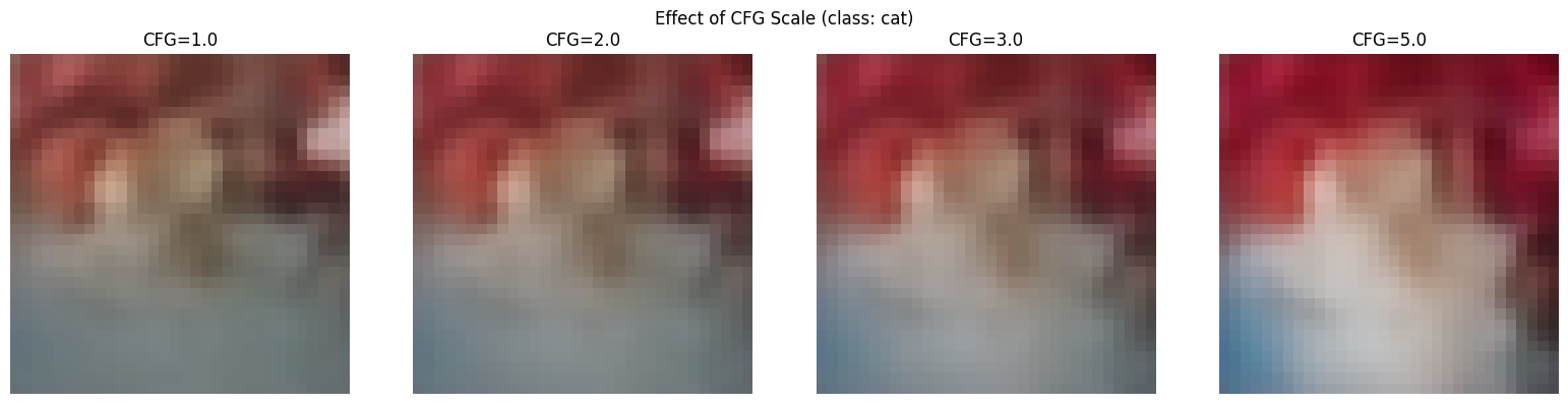

Higher CFG → stronger class adherence
Too high → less diversity, potential artifacts

Part 7: The Efficiency Win¶

Let’s quantify the computational advantage.

import time

num_samples = 16
num_steps = 50

# Latent diffusion timing
torch.cuda.synchronize() if torch.cuda.is_available() else None
start = time.time()

with torch.no_grad():
    _ = sample_latent(
        model=latent_dit,
        vae=vae,
        num_samples=num_samples,
        latent_shape=(4, 8, 8),
        num_steps=num_steps,
        device=device,
    )

torch.cuda.synchronize() if torch.cuda.is_available() else None
latent_time = time.time() - start

print(f"Latent Diffusion: {num_samples} samples, {num_steps} steps")
print(f"  Total time: {latent_time:.2f}s")
print(f"  Per image: {latent_time/num_samples*1000:.1f}ms")
print()
print("Breakdown:")
print(f"  ODE steps: {num_steps} × {num_samples} = {num_steps * num_samples} DiT forward passes")
print(f"  Each on 16 tokens (256 attention pairs)")
print(f"  VAE decode: {num_samples} passes (once at the end)")

Latent Diffusion: 16 samples, 50 steps
  Total time: 0.11s
  Per image: 7.0ms

Breakdown:
  ODE steps: 50 × 16 = 800 DiT forward passes
  Each on 16 tokens (256 attention pairs)
  VAE decode: 16 passes (once at the end)

Summary: The Complete Latent Diffusion Architecture¶

The Big Picture¶

TRAINING:
  Image x ──[VAE Encode]──> z₀ ──[interpolate with noise]──> z_t ──[DiT]──> v̂
                                                                      │
                                              Loss = ║v̂ - (z₁ - z₀)║²

INFERENCE:
  Noise z₁ ──[DiT + ODE integration]──> z₀ ──[VAE Decode]──> Image x

Key Equations¶

Component	Equation	Purpose
VAE Encode	$z = \mu + \sigma \epsilon$	Compress to latent
VAE Decode	$\hat{x} = D(z)$	Reconstruct image
VAE Loss	$\mathcal{L} = \|x-\hat{x}\|^2 + \beta D_{KL}$	Train compression
Interpolation	$z_t = (1-t)z_0 + tz_1$	Flow path in latent space
Target velocity	$v = z_1 - z_0$	What DiT predicts
Training loss	$\mathcal{L} = \|v_\theta(z_t, t) - v\|^2$	Train DiT
Generation ODE	$\frac{dz}{dt} = -v_\theta(z_t, t)$	Integrate from noise

Compression Ratios in Practice¶

Image Size	Pixel Dims	Latent Dims (8× spatial)	Compression
32×32×3	3,072	4×4×4 = 64	48×
64×64×3	12,288	8×8×4 = 256	48×
256×256×3	196,608	32×32×4 = 4,096	48×
512×512×3	786,432	64×64×4 = 16,384	48×

(Our CIFAR-10 VAE uses 4× spatial compression, so 12× total.)

Why Latent Diffusion Works¶

Perceptual compression: VAEs compress semantically—nearby latents decode to similar images
High-frequency details: The decoder handles fine details; the diffusion model only needs coarse structure
Computational efficiency: 48× fewer dimensions → orders of magnitude faster
Same quality: With a good VAE, no perceptual quality loss

This Is Stable Diffusion¶

You’ve now implemented the core of Stable Diffusion:

Component	Stable Diffusion	Our Implementation
Autoencoder	KL-VAE (pretrained)	SmallVAE
Denoiser	U-Net (or DiT in SD3)	DiT
Text encoder	CLIP	(Notebook 04)
Conditioning	Cross-attention	adaLN / Cross-attention
Sampling	DDPM/DDIM/DPM++	Euler ODE

The architecture is the same. Stable Diffusion just scales everything up:

Larger VAE (trained on millions of images)
Larger U-Net/DiT (billions of parameters)
CLIP trained on 400M image-text pairs

Congratulations! You understand the complete text-to-image pipeline from first principles.

# Save trained models
vae_trainer.save_checkpoint("phase5_vae.pt")
latent_trainer.save_checkpoint("phase5_latent_dit.pt")
cond_latent_trainer.save_checkpoint("phase5_cond_latent_dit.pt")

print("Models saved:")
print("  - phase5_vae.pt")
print("  - phase5_latent_dit.pt")
print("  - phase5_cond_latent_dit.pt")

Models saved:
  - phase5_vae.pt
  - phase5_latent_dit.pt
  - phase5_cond_latent_dit.pt