
In the previous notebook, we controlled generation with discrete class labels (0-9 for digits). This required a fixed vocabulary and a simple embedding table. Now we move to natural language conditioning - the ability to say “a photo of a cat” and generate a cat.
This is how modern text-to-image models like Stable Diffusion, DALL-E, and Midjourney work.
The Evolution of Conditioning
| Notebook | Conditioning | Example | Mechanism |
|---|---|---|---|
| Flow Matching, DiT | None | Generate any image | - |
| Class Conditioning | Class label | “Generate digit 7” | |
| This Notebook | Text prompt | “a photo of a cat” | Cross-attention to CLIP |
The Mathematical Challenge
We need to learn a text-conditional velocity field:
But “String” isn’t a mathematical object. We need to convert text to vectors.
Why Cross-Attention?
In the previous notebook, we simply added the class embedding to the timestep embedding:
This works for single tokens (class labels), but text has multiple tokens. We need a mechanism that:
Handles variable-length sequences
Allows different image regions to focus on different words
Preserves the full information in each token
Cross-attention provides all of this.
What We’ll Learn
CLIP Text Encoder - How text becomes vectors
Cross-Attention - How image patches attend to text tokens
Text-Conditional DiT - The full architecture
CFG for Text - Classifier-free guidance with prompts
import torch
import torch.nn as nn
import torchvision
import torchvision.transforms as transforms
from torch.utils.data import DataLoader
import matplotlib.pyplot as plt
import numpy as np

%load_ext autoreload
%autoreload 2

from from_noise_to_images import get_device
device = get_device()
print(f"Using device: {device}")
Using device: cuda
Step 1: CLIP - The Bridge Between Text and Images
CLIP (Contrastive Language-Image Pre-training) is a model trained on 400M image-text pairs to learn a shared embedding space.
The CLIP Training Objective
Given a batch of image-text pairs, CLIP learns to:
Maximize similarity between matching pairs
Minimize similarity between non-matching pairs
This creates visually grounded text embeddings:
| Property | Meaning | Example |
|---|---|---|
| Semantic | Similar meanings → similar vectors | “dog” ≈ “puppy” |
| Visual | Vectors encode visual features | “red” encodes color |
| Compositional | Combinations work | “blue dog” is meaningful |
CLIP Text Encoder Architecture
Text: "a photo of a cat"
         │
         ▼
    ┌─────────┐
    │ Tokenize│  → ["a", "photo", "of", "a", "cat"]
    └────┬────┘
         │
         ▼
    ┌─────────┐
    │  Embed  │  → [e₁, e₂, e₃, e₄, e₅]
    └────┬────┘
         │
         ▼
    ┌─────────────┐
    │ Transformer │  → 12 layers of self-attention
    └──────┬──────┘
           │
           ▼
    Token Embeddings: Z ∈ R^{M × D}
We use the token embeddings (not just the pooled output) for cross-attention.
from from_noise_to_images.text_encoder import CLIPTextEncoder

# Load CLIP text encoder
text_encoder = CLIPTextEncoder(
    model_name="openai/clip-vit-base-patch32",
    device=device,
)

print(f"CLIP embedding dimension: {text_encoder.embed_dim}")
print(f"Max sequence length: {text_encoder.max_length}")
CLIP embedding dimension: 512
Max sequence length: 77
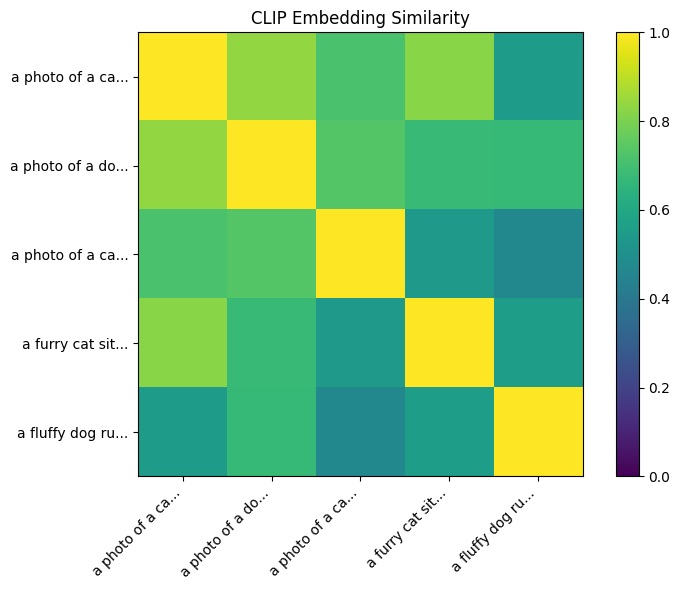
# Explore CLIP embeddings
prompts = [
    "a photo of a cat",
    "a photo of a dog",
    "a photo of a car",
    "a furry cat sitting",
    "a fluffy dog running",
]

# Get token embeddings and pooled embeddings
token_embeddings, pooled = text_encoder.encode(prompts, return_pooled=True)

print(f"Token embeddings shape: {token_embeddings.shape}")
print(f"  → (batch_size, max_length, embed_dim)")
print(f"Pooled embeddings shape: {pooled.shape}")
print(f"  → (batch_size, embed_dim)")

# Compute similarity matrix from pooled embeddings
pooled_norm = pooled / pooled.norm(dim=-1, keepdim=True)
similarity = (pooled_norm @ pooled_norm.T).cpu().numpy()

# Visualize
fig, ax = plt.subplots(figsize=(8, 6))
im = ax.imshow(similarity, cmap='viridis', vmin=0, vmax=1)
ax.set_xticks(range(len(prompts)))
ax.set_yticks(range(len(prompts)))
ax.set_xticklabels([p[:15] + "..." for p in prompts], rotation=45, ha='right')
ax.set_yticklabels([p[:15] + "..." for p in prompts])
ax.set_title('CLIP Embedding Similarity')
plt.colorbar(im)
plt.tight_layout()
plt.show()

print("\nKey Observations:")
print("  - 'cat' prompts are similar to each other")
print("  - 'dog' prompts are similar to each other")
print("  - Both are less similar to 'car'")
Token embeddings shape: torch.Size([5, 77, 512])
→ (batch_size, max_length, embed_dim)
Pooled embeddings shape: torch.Size([5, 512])
→ (batch_size, embed_dim)
Key Observations:
  - 'cat' prompts are similar to each other
  - 'dog' prompts are similar to each other
  - Both are less similar to 'car'
Step 2: Cross-Attention - Image Patches Attending to Text
Cross-attention allows each image patch to “look at” the text and extract relevant information.
Mathematical Formulation
Given:
Image patch embeddings: (N patches)
Text token embeddings: (M tokens)
Cross-attention computes:
where:
. Queries from image patches
. Keys from text tokens
. Values from text tokens
The Attention Matrix
Entry represents: “How much should image patch attend to text token ?”
Intuitive Understanding
For the prompt “a RED dog RUNNING”:
                    Text Tokens
                 a   RED  dog  RUNNING
              ┌────────────────────────┐
    Patch 1   │ 0.1  0.7  0.1   0.1    │  ← Color region, attends to "RED"
    Patch 2   │ 0.1  0.1  0.6   0.2    │  ← Body region, attends to "dog"
    Patch 3   │ 0.1  0.1  0.3   0.5    │  ← Leg region, attends to "RUNNING"
    Patch 4   │ 0.2  0.3  0.3   0.2    │  ← Background, mixed attention
              └────────────────────────┘
Self-Attention vs Cross-Attention
| Aspect | Self-Attention | Cross-Attention |
|---|---|---|
| Q, K, V source | Same sequence (X) | Q from X, K/V from Z |
| Attention shape | ||
| Purpose | Patch-to-patch relations | Text-to-image transfer |
| Information flow | Within image | From text to image |
from from_noise_to_images.dit import CrossAttention

# Create a cross-attention layer
embed_dim = 256   # Image patch embedding dimension
context_dim = 512  # CLIP text embedding dimension
num_heads = 8

cross_attn = CrossAttention(
    embed_dim=embed_dim,
    context_dim=context_dim,
    num_heads=num_heads,
).to(device)

# Simulate inputs
batch_size = 2
num_patches = 64  # 8x8 grid
num_tokens = 10   # Text sequence length

# Random image patch embeddings
x = torch.randn(batch_size, num_patches, embed_dim, device=device)

# Random text embeddings (simulating CLIP output)
context = torch.randn(batch_size, num_tokens, context_dim, device=device)

# Forward pass
with torch.no_grad():
    output = cross_attn(x, context)

print(f"Cross-Attention Dimensions:")
print(f"  Image patches (X): {x.shape}")
print(f"  Text tokens (Z):   {context.shape}")
print(f"  Output:            {output.shape}")
print(f"\nThe output has the same shape as the image patches!")
print(f"Each patch now contains information from relevant text tokens.")
Cross-Attention Dimensions:
Image patches (X): torch.Size([2, 64, 256])
Text tokens (Z): torch.Size([2, 10, 512])
Output: torch.Size([2, 64, 256])
The output has the same shape as the image patches!
Each patch now contains information from relevant text tokens.
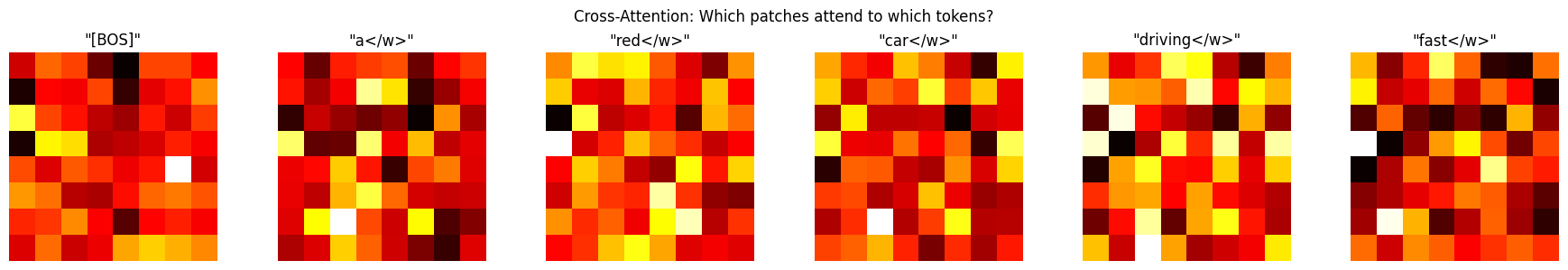
# Visualize attention weights for a real prompt
def visualize_cross_attention_weights(
    cross_attn: CrossAttention,
    x: torch.Tensor,
    context: torch.Tensor,
    tokens: list,
):
    """Visualize what each image patch attends to in the text."""
    B, N, _ = x.shape
    M = context.shape[1]
    H = cross_attn.num_heads
    d = cross_attn.head_dim

    with torch.no_grad():
        # Compute Q, K
        q = cross_attn.q_proj(x)
        k = cross_attn.k_proj(context)

        # Reshape for attention
        q = q.view(B, N, H, d).transpose(1, 2)
        k = k.view(B, M, H, d).transpose(1, 2)

        # Compute attention scores
        attn = (q @ k.transpose(-2, -1)) * cross_attn.scale
        attn = attn.softmax(dim=-1)  # (B, H, N, M)

    # Average over heads and batch
    attn_avg = attn[0].mean(dim=0).cpu().numpy()  # (N, M)

    # Reshape to 2D grid (assuming square patches)
    grid_size = int(np.sqrt(N))

    # Plot attention for each token
    num_tokens_to_show = min(6, M)
    fig, axes = plt.subplots(1, num_tokens_to_show, figsize=(3*num_tokens_to_show, 3))

    for i in range(num_tokens_to_show):
        attn_map = attn_avg[:, i].reshape(grid_size, grid_size)
        axes[i].imshow(attn_map, cmap='hot')
        token = tokens[i] if i < len(tokens) else "[PAD]"
        axes[i].set_title(f'"{token}"')
        axes[i].axis('off')

    plt.suptitle('Cross-Attention: Which patches attend to which tokens?', fontsize=12)
    plt.tight_layout()
    plt.show()

# Get real CLIP embeddings
test_prompt = "a red car driving fast"
test_embeddings, test_mask = text_encoder(test_prompt)
test_embeddings = test_embeddings.to(device)

# Get tokens for visualization
tokens = text_encoder.tokenizer.tokenize(test_prompt)
tokens = ['[BOS]'] + tokens + ['[EOS]']

# Random image patches (in practice, these would be from the DiT)
num_patches = 64
x_test = torch.randn(1, num_patches, embed_dim, device=device)

print(f"Prompt: '{test_prompt}'")
print(f"Tokens: {tokens}")
print()

visualize_cross_attention_weights(cross_attn, x_test, test_embeddings, tokens)
Prompt: 'a red car driving fast'
Tokens: ['[BOS]', 'a</w>', 'red</w>', 'car</w>', 'driving</w>', 'fast</w>', '[EOS]']
Step 3: Text-Conditional DiT Architecture
The TextConditionalDiT extends our DiT with cross-attention layers.
Block Structure
Each TextConditionedDiTBlock has three components:
                                        Text Embeddings Z
                                              │
                                              ▼
x ─► adaLN ─► Self-Attn ─► + ─► adaLN ─► Cross-Attn ─► + ─► adaLN ─► MLP ─► + ─► out
│                         │   │                        │   │                │
└───────(residual)────────┘   └───────(residual)───────┘   └──(residual)────┘
Mathematical Formulation
Let be the input to layer , be timestep conditioning, be text embeddings:
Full Architecture
Text Prompt                    Noisy Image x_t          Timestep t
     │                              │                       │
     ▼                              ▼                       ▼
┌─────────┐                  ┌───────────┐           ┌───────────┐
│  CLIP   │                  │ Patchify  │           │ Time Emb  │
│ Encoder │                  │ + PosEmb  │           │   (MLP)   │
└────┬────┘                  └─────┬─────┘           └─────┬─────┘
     │                             │                       │
     │ Z ∈ R^{M × D}               │ X ∈ R^{N × d}         │ c ∈ R^{d_c}
     │                             │                       │
     │                             ▼                       │
     │                    ┌─────────────────┐              │
     └───────────────────►│ TextConditioned │◄─────────────┘
                          │    DiT Blocks   │
                          └────────┬────────┘
                                   │
                                   ▼
                          ┌─────────────────┐
                          │   Unpatchify    │
                          └────────┬────────┘
                                   │
                                   ▼
                          Velocity v ∈ R^{C × H × W}
Key Differences from ConditionalDiT
| Aspect | ConditionalDiT | TextConditionalDiT |
|---|---|---|
| Conditioning | Class labels (0-9) | Text prompts |
| Embedding | Learnable table | Frozen CLIP |
| Integration | Added to timestep | Cross-attention |
| Vocabulary | Fixed (10 classes) | Open (any text) |
| Representation | Single vector | Sequence of tokens |
from from_noise_to_images.dit import TextConditionalDiT

# Create the text-conditional DiT for CIFAR-10 (32x32 RGB)
model = TextConditionalDiT(
    img_size=32,          # CIFAR-10 image size
    patch_size=4,         # 4x4 patches → 8x8 = 64 patches
    in_channels=3,        # RGB
    embed_dim=256,        # Patch embedding dimension
    depth=6,              # Number of transformer blocks
    num_heads=8,          # Attention heads
    mlp_ratio=4.0,        # MLP expansion
    context_dim=512,      # CLIP ViT-B/32 embedding dimension
).to(device)

# Count parameters
num_params = sum(p.numel() for p in model.parameters() if p.requires_grad)
print(f"TextConditionalDiT Parameters: {num_params:,}")

# Compare to ConditionalDiT
from from_noise_to_images.dit import ConditionalDiT
class_model = ConditionalDiT(img_size=32, patch_size=4, in_channels=3)
class_params = sum(p.numel() for p in class_model.parameters() if p.requires_grad)
print(f"ConditionalDiT Parameters: {class_params:,}")
print(f"Difference: +{num_params - class_params:,} (cross-attention layers)")
TextConditionalDiT Parameters: 18,145,072
ConditionalDiT Parameters: 12,379,440
Difference: +5,765,632 (cross-attention layers)
# Test forward pass
batch_size = 4

# Random noisy images
x = torch.randn(batch_size, 3, 32, 32, device=device)

# Random timesteps
t = torch.rand(batch_size, device=device)

# Text embeddings from CLIP
prompts = [
    "a photo of a cat",
    "a photo of a dog",
    "a photo of a car",
    "a photo of a plane",
]
text_embeddings, text_mask = text_encoder(prompts)
text_embeddings = text_embeddings.to(device)
text_mask = text_mask.to(device)

# Forward pass
with torch.no_grad():
    v_pred = model(x, t, text_embeddings, text_mask)

print(f"Input shape:       {x.shape}")
print(f"Timesteps shape:   {t.shape}")
print(f"Text embed shape:  {text_embeddings.shape}")
print(f"Text mask shape:   {text_mask.shape}")
print(f"Output shape:      {v_pred.shape}")
print(f"\nModel correctly outputs velocity field with same shape as input!")
Input shape: torch.Size([4, 3, 32, 32])
Timesteps shape: torch.Size([4])
Text embed shape: torch.Size([4, 77, 512])
Text mask shape: torch.Size([4, 77])
Output shape: torch.Size([4, 3, 32, 32])
Model correctly outputs velocity field with same shape as input!
Step 4: Dataset - CIFAR-10 with Text Captions
We’ll use CIFAR-10 (32×32 RGB images) with class names converted to captions.
CIFAR-10 Classes → Captions
| Index | Class | Caption Template |
|---|---|---|
| 0 | airplane | “a photo of an airplane” |
| 1 | automobile | “a photo of an automobile” |
| 2 | bird | “a photo of a bird” |
| 3 | cat | “a photo of a cat” |
| 4 | deer | “a photo of a deer” |
| 5 | dog | “a photo of a dog” |
| 6 | frog | “a photo of a frog” |
| 7 | horse | “a photo of a horse” |
| 8 | ship | “a photo of a ship” |
| 9 | truck | “a photo of a truck” |
CLIP understands “a photo of a X” format very well from its training.
from from_noise_to_images.text_encoder import make_cifar10_captions

# Load CIFAR-10
transform = transforms.Compose([
    transforms.ToTensor(),
    transforms.Normalize((0.5, 0.5, 0.5), (0.5, 0.5, 0.5))  # [-1, 1]
])

train_dataset = torchvision.datasets.CIFAR10(
    root="./data",
    train=True,
    download=True,
    transform=transform
)

train_loader = DataLoader(
    train_dataset,
    batch_size=64,
    shuffle=True,
    num_workers=0,
    drop_last=True
)

# Test caption function
sample_labels = torch.tensor([0, 3, 5, 8])
captions = make_cifar10_captions(sample_labels)

print("Label → Caption mapping:")
for label, caption in zip(sample_labels.tolist(), captions):
    print(f"  {label} → '{caption}'")
Label → Caption mapping:
0 → 'a photo of an airplane'
3 → 'a photo of a cat'
5 → 'a photo of a dog'
8 → 'a photo of a ship'
C:\Users\zhube\Code\intro-to-transformers\.venv\Lib\site-packages\torchvision\datasets\cifar.py:83: VisibleDeprecationWarning: dtype(): align should be passed as Python or NumPy boolean but got `align=0`. Did you mean to pass a tuple to create a subarray type? (Deprecated NumPy 2.4)
  entry = pickle.load(f, encoding="latin1")
# Visualize samples with their captions
images, labels = next(iter(train_loader))
captions = make_cifar10_captions(labels[:8])

fig, axes = plt.subplots(2, 4, figsize=(12, 6))

for i, (ax, img, caption) in enumerate(zip(axes.flat, images[:8], captions)):
    # Denormalize
    img = (img + 1) / 2
    img = img.permute(1, 2, 0).numpy()
    img = np.clip(img, 0, 1)

    ax.imshow(img)
    ax.set_title(caption, fontsize=9)
    ax.axis('off')

plt.suptitle('CIFAR-10 Samples with Text Captions', fontsize=12)
plt.tight_layout()
plt.show()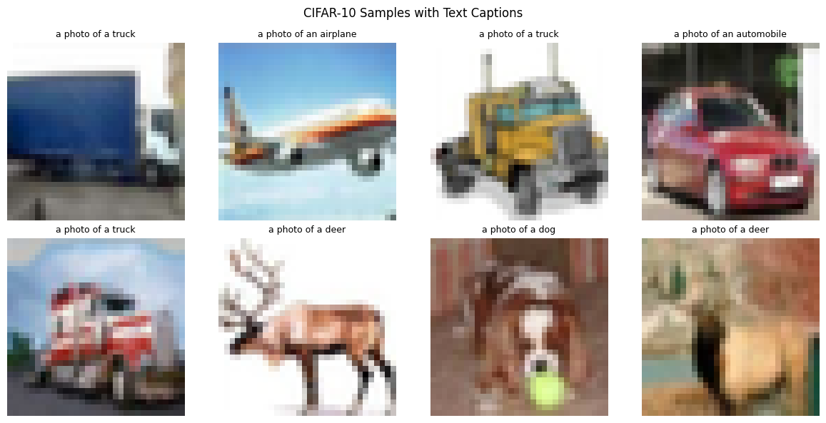
Step 5: Classifier-Free Guidance for Text
CFG works the same way as before, but with text embeddings.
The CFG Formula (Same as Before)
where:
. Velocity with text embedding
. Velocity with null text
. Guidance scale
What is Null Text?
The “null text” is an empty string encoded by CLIP:
This represents “no specific content” - similar to the null class in the previous notebook.
Text Dropout During Training
To enable CFG, we randomly replace text embeddings with null:
Typically (10%).
Guidance Scale: Text vs Class
| Conditioning | Typical Scale | Reason |
|---|---|---|
| Class | 3-5 | Simple, direct mapping |
| Text | 7-10 | Complex, needs stronger push |
Text conditioning is more nuanced - higher guidance pushes toward the most “on-prompt” outputs.
# Compare text embedding vs null embedding
_, text_emb = text_encoder.encode(["a photo of a cat"], return_pooled=True)
_, null_emb = text_encoder.encode([""], return_pooled=True)

# Compute similarity
text_norm = text_emb / text_emb.norm(dim=-1, keepdim=True)
null_norm = null_emb / null_emb.norm(dim=-1, keepdim=True)
similarity = (text_norm @ null_norm.mT).item()

print(f"Text embedding shape: {text_emb.shape}")
print(f"Null embedding shape: {null_emb.shape}")
print(f"Cosine similarity: {similarity:.3f}")
print(f"\nThe null embedding is different from any real text embedding.")
print(f"This makes CFG work: we can push away from 'nothing' toward 'something'.")
Text embedding shape: torch.Size([1, 512])
Null embedding shape: torch.Size([1, 512])
Cosine similarity: 0.653
The null embedding is different from any real text embedding.
This makes CFG work: we can push away from 'nothing' toward 'something'.
Step 6: Training the Text-Conditional DiT
Training follows the same flow matching objective, now with text conditioning.
Training Algorithm
For each batch of (image, label) pairs:
Convert labels to captions:
Encode with CLIP:
Apply text dropout: With 10% probability,
Sample noise and time: ,
Interpolate:
Predict velocity:
Compute loss:
Loss Function
from from_noise_to_images.train import TextConditionalTrainer

# Create the trainer
trainer = TextConditionalTrainer(
    model=model,
    text_encoder=text_encoder,
    dataloader=train_loader,
    caption_fn=make_cifar10_captions,
    lr=1e-4,
    weight_decay=0.01,
    text_drop_prob=0.1,  # 10% text dropout for CFG
    device=device,
)

print("Training Text-Conditional DiT with CFG text dropout...")
print("(10% of samples trained with null text)\n")

NUM_EPOCHS = 30
losses = trainer.train(num_epochs=NUM_EPOCHS)
Training Text-Conditional DiT with CFG text dropout...
(10% of samples trained with null text)
Training on cuda
Model parameters: 18,145,072
CFG text dropout: 10%
Epoch 1: avg_loss = 0.5515
Epoch 2: avg_loss = 0.2989
Epoch 3: avg_loss = 0.2803
Epoch 4: avg_loss = 0.2667
Epoch 5: avg_loss = 0.2587
Epoch 6: avg_loss = 0.2521
Epoch 7: avg_loss = 0.2478
Epoch 8: avg_loss = 0.2423
Epoch 9: avg_loss = 0.2383
Epoch 10: avg_loss = 0.2362
Epoch 11: avg_loss = 0.2341
Epoch 12: avg_loss = 0.2294
Epoch 13: avg_loss = 0.2254
Epoch 14: avg_loss = 0.2235
Epoch 15: avg_loss = 0.2208
Epoch 16: avg_loss = 0.2192
Epoch 17: avg_loss = 0.2162
Epoch 18: avg_loss = 0.2144
Epoch 19: avg_loss = 0.2121
Epoch 20: avg_loss = 0.2092
Epoch 21: avg_loss = 0.2088
Epoch 22: avg_loss = 0.2074
Epoch 23: avg_loss = 0.2064
Epoch 24: avg_loss = 0.2048
Epoch 25: avg_loss = 0.2035
Epoch 26: avg_loss = 0.2014
Epoch 27: avg_loss = 0.2015
Epoch 28: avg_loss = 0.2014
Epoch 29: avg_loss = 0.2009
Epoch 30: avg_loss = 0.2001
# Plot training loss
plt.figure(figsize=(10, 4))
plt.plot(losses)
plt.xlabel('Epoch')
plt.ylabel('Loss')
plt.title('Text-Conditional DiT Training Loss')
plt.grid(True, alpha=0.3)
plt.show()

print(f"Final loss: {losses[-1]:.4f}")
Final loss: 0.2001
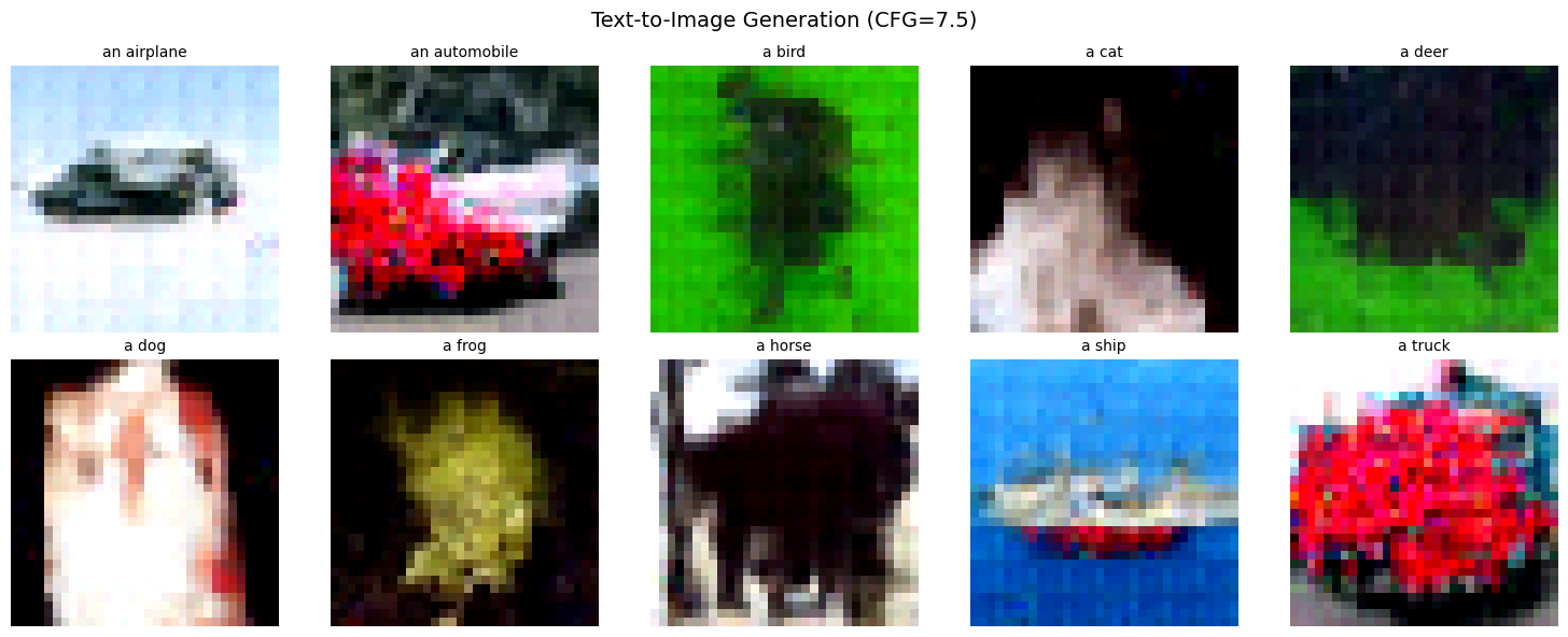
Step 7: Sampling with Text Prompts
Now the exciting part - generating images from text!
CFG Sampling Algorithm
Input: Trained model v_θ, text prompt, guidance scale w, num_steps N

1. Encode text: Z_text = CLIP(prompt)
2. Encode null: Z_null = CLIP("")
3. Sample x_1 ~ N(0, I)  # Pure noise
4. dt = 1/N

For t = 1, 1-dt, ..., dt:
    v_cond = v_θ(x_t, t, Z_text)    # With text
    v_uncond = v_θ(x_t, t, Z_null)  # Without text
    v_guided = v_uncond + w × (v_cond - v_uncond)  # CFG
    x_t ← x_t - dt × v_guided       # Euler step

Return x_0  # Generated image
from from_noise_to_images.sampling import sample_text_conditional
model.eval()
# Generate images for each CIFAR-10 class
prompts = [
"a photo of an airplane",
"a photo of an automobile",
"a photo of a bird",
"a photo of a cat",
"a photo of a deer",
"a photo of a dog",
"a photo of a frog",
"a photo of a horse",
"a photo of a ship",
"a photo of a truck",
]
print("Generating images for each class with CFG scale=7.5...")
samples = sample_text_conditional(
model=model,
text_encoder=text_encoder,
prompts=prompts,
image_shape=(3, 32, 32),
num_steps=50,
cfg_scale=7.5,
device=device,
)
# Display results
fig, axes = plt.subplots(2, 5, figsize=(15, 6))
for i, (ax, prompt) in enumerate(zip(axes.flat, prompts)):
img = (samples[i] + 1) / 2 # Denormalize
img = img.permute(1, 2, 0).cpu().numpy()
img = np.clip(img, 0, 1)
ax.imshow(img)
ax.set_title(prompt.replace('a photo of ', ''), fontsize=10)
ax.axis('off')
plt.suptitle('Text-to-Image Generation (CFG=7.5)', fontsize=14)
plt.tight_layout()
plt.show()Generating images for each class with CFG scale=7.5...
# Compare different CFG scales
test_prompt = "a photo of a cat"
cfg_scales = [1.0, 3.0, 5.0, 7.5, 10.0, 15.0]

print(f"Comparing CFG scales for: '{test_prompt}'")

fig, axes = plt.subplots(1, len(cfg_scales), figsize=(18, 3))

for ax, scale in zip(axes, cfg_scales):
    # Use same seed for fair comparison
    torch.manual_seed(42)

    sample = sample_text_conditional(
        model=model,
        text_encoder=text_encoder,
        prompts=[test_prompt],
        image_shape=(3, 32, 32),
        num_steps=50,
        cfg_scale=scale,
        device=device,
    )

    img = (sample[0] + 1) / 2
    img = img.permute(1, 2, 0).cpu().numpy()
    img = np.clip(img, 0, 1)

    ax.imshow(img)
    ax.set_title(f'scale={scale}')
    ax.axis('off')

plt.suptitle(f'Effect of CFG Scale: "{test_prompt}"', fontsize=12)
plt.tight_layout()
plt.show()

print("\nObservations:")
print("  scale=1.0: No guidance, blurry")
print("  scale=3-5: Mild guidance, improving")
print("  scale=7-10: Good balance")
print("  scale=15+: May oversaturate")
Comparing CFG scales for: 'a photo of a cat'
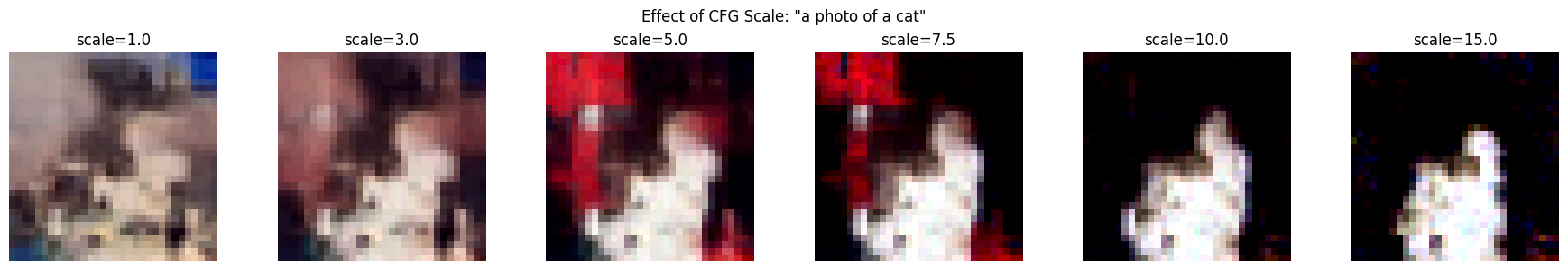
Observations:
  scale=1.0: No guidance, blurry
  scale=3-5: Mild guidance, improving
  scale=7-10: Good balance
  scale=15+: May oversaturate
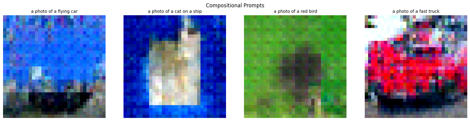
# Try some creative prompts
creative_prompts = [
    "a photo of a flying car",
    "a photo of a cat on a ship",
    "a photo of a red bird",
    "a photo of a fast truck",
]

print("Testing compositional understanding...")
print("(Results may be limited by CIFAR-10 training data)\n")

torch.manual_seed(123)
creative_samples = sample_text_conditional(
    model=model,
    text_encoder=text_encoder,
    prompts=creative_prompts,
    image_shape=(3, 32, 32),
    num_steps=50,
    cfg_scale=7.5,
    device=device,
)

fig, axes = plt.subplots(1, 4, figsize=(16, 4))

for ax, prompt, sample in zip(axes, creative_prompts, creative_samples):
    img = (sample + 1) / 2
    img = img.permute(1, 2, 0).cpu().numpy()
    img = np.clip(img, 0, 1)

    ax.imshow(img)
    ax.set_title(prompt, fontsize=10)
    ax.axis('off')

plt.suptitle('Compositional Prompts', fontsize=12)
plt.tight_layout()
plt.show()
Testing compositional understanding...
(Results may be limited by CIFAR-10 training data)
# Save the trained model
trainer.save_checkpoint("phase4_text_conditional_dit.pt")
print("Model saved to phase4_text_conditional_dit.pt")
Model saved to phase4_text_conditional_dit.pt
Summary: Text-to-Image Generation
We extended the DiT to accept natural language prompts via CLIP and cross-attention.
Key Equations
| Concept | Equation |
|---|---|
| CLIP encoding | |
| Cross-attention | |
| Queries | (from image patches) |
| Keys, Values | , (from text tokens) |
| Training loss | |
| CFG formula | |
| Null text |
Cross-Attention Details
The attention matrix :
= number of image patches
= number of text tokens
answers: “How much should image patch attend to text token ?”
Architecture Comparison
| Notebook | Model | Conditioning | Mechanism |
|---|---|---|---|
| 01-02 | DiT | None | - |
| 03 | ConditionalDiT | Class labels | , adaLN |
| 04 | TextConditionalDiT | Text prompts | Cross-attention to CLIP |
What’s Next
In the next notebook, we add latent space diffusion with a VAE:
| Current (Pixel Space) | Next (Latent Space) |
|---|---|
| Diffusion on 32×32×3 | Diffusion on 4×4×4 latent |
| 3,072 dimensions | 64 dimensions (48× smaller) |
| Limited resolution | Scales to 256×256+ |
This is how Stable Diffusion achieves high-resolution generation!